Omix - Pseudotemporal multi-omics integration • Omix

Overview

The goal of Omix is to provide tools in R to build a complete analysis workflow for integrative analysis of data generated from multi-omics platform.

Generate a multi-omics object using MultiAssayExperiment.
Quality control of single-omics data.
Formatting, normalisation, denoising of single-omics data.
Separate single-omics analyses.
Integration of multi-omics data for combined analysis.
Publication quality plots and interactive analysis reports based of shinyApp.

Currently, Omix supports the integration of bulk transcriptomics and bulk proteomics.

Running Omix

The Omix pipeline requires the following input:

rawdata_rna: A data-frame containing raw RNA count with rownames as gene and colnames as samples.
rawdata_protein: A data-frame containing protein abundance with rownames as proteins and colnames as samples.
map_rna: A data-frame of two columns named primary and colname where primary should contain unique sample name with a link to sample metadata and colname is the column names of the rawdata_rna data-frame.
map_protein: A data-frame of two columns named primary and colname where primary should contain unique sample name with a link to sample metadata and colname is the column names of the rawdata_protein data-frame.
metadata_rna: A data-frame containing rna assay specific metadata where rownames are same as the colnames of rawdata_rna data.frame.
metadata_protein: A data-frame containing protein assay specific metadata where rownames are same as the colnames of rawdata_protein data.frame.
individual_metadata: A data-frame containing individual level metadata for both omics assays.

Call required packages for vignette:

library(Omix)
library(purrr)
library(ggplot2)
library(dplyr)
library(synapser)
library(tibble)

First we must load the data from Omix for the vignette:

outputDir <- tempdir()
ctd_fp <-file.path(outputDir, "ctd.rds")
ensembl_fp  <-file.path(outputDir, "ensembl.rds")
TF_fp <- file.path(outputDir, "Enrichr_Queries.gmt.txt")
GO_fp <- file.path(outputDir, "GO_Biological_Process_2021.txt")


download.file(url = "https://raw.githubusercontent.com/eleonore-schneeg/OmixData/main/ctd-2.rds",destfile=ctd_fp)

download.file(url = "https://raw.githubusercontent.com/eleonore-schneeg/OmixData/main/ensembl_mappings_human.tsv",destfile=ensembl_fp)

download.file(url = "https://raw.githubusercontent.com/eleonore-schneeg/OmixData/main/Enrichr_Queries.gmt.txt",destfile=TF_fp)

download.file(url = "https://raw.githubusercontent.com/eleonore-schneeg/OmixData/main/GO_Biological_Process_2021.txt",destfile=GO_fp)


synapser::synLogin(email=Sys.getenv("SYNAPSE_ID"), authToken=Sys.getenv("AUTHTOKEN"))

Welcome, ems2817!NULL

rawdata_rna <- read.csv(synapser::synGet('syn51516100')$path, header=T, stringsAsFactors = F, row.names=1)
rawdata_protein <- read.csv(synapser::synGet('syn51516105')$path, header=T, stringsAsFactors = F, row.names=1)
map_rna <-read.csv(synapser::synGet('syn51516102')$path, header=T, stringsAsFactors = F, row.names=1)
map_prot <- read.csv(synapser::synGet('syn51516104')$path, header=T, stringsAsFactors = F, row.names=1)
metadata_rna<-read.csv(synapser::synGet('syn51516103')$path, header=T, stringsAsFactors = F, row.names=1)
metadata_prot <- read.csv(synapser::synGet('syn51516106')$path, header=T, stringsAsFactors = F, row.names=1)
individual_metadata <-read.csv(synapser::synGet('syn51516101')$path, header=T, stringsAsFactors = F, row.names=1)
clusters<-readRDS(synapser::synGet('syn51516107')$path)
integrative_model<-readRDS(synapser::synGet('syn51520491')$path)

ctd <-  readRDS(paste0(outputDir,'/ctd.rds'))
ensembl <-read.delim(file=paste0(outputDir,'/ensembl.rds'), sep = '\t', header = TRUE)
rna_qc_data_matrix <- NULL

Sanity check

all(rownames(metadata_rna) == colnames(rawdata_rna))

## [1] TRUE

all(rownames(metadata_prot) == colnames(rawdata_protein))

## [1] TRUE

Raw rna counts

rawdata_rna is a data-frame of raw counts, with features as rows and samples as columns

print(rawdata_rna[1:5,1:5])

##                 IGF117745 IGF117748 IGF117756 IGF117758 IGF117759
## ENSG00000223972         0         0         1         0         1
## ENSG00000227232        23        26        40        26        30
## ENSG00000278267         7         5         1         4         0
## ENSG00000243485         0         0         0         1         0
## ENSG00000284332         0         0         0         0         0

Raw protein abundance

rawdata_protein is a data-frame of raw protein abundances, with features as rows and samples as columns

print(rawdata_protein[10:15,10:15])

##                    BBN_16213_SOM_P2WH4_001 BBN_18399_MTG_P2WF5_001
## MAP1LC3B;MAP1LC3B2               140.21600                118.1090
## PGP                               33.91880                 24.3759
## BTBD17                                  NA                      NA
## WIPF3                             39.10300                 98.0357
## IGLON5                             8.55527                 10.2548
## TUBAL3                          9432.14000              10277.5000
##                    BBN_18399_SOM_P2WF6_001 BBN_18813_SOM_P3WB2_001
## MAP1LC3B;MAP1LC3B2                116.8410               109.55500
## PGP                                15.2674                31.62250
## BTBD17                             13.8635                      NA
## WIPF3                              68.9909                26.42480
## IGLON5                             21.7657                 8.52512
## TUBAL3                           9565.3200             10144.50000
##                    BBN_19214_MTG_P2WA3_001 BBN_19214_SOM_P2WA4_001
## MAP1LC3B;MAP1LC3B2                121.1260                166.2360
## PGP                                18.2978                 26.0274
## BTBD17                                  NA                 17.6870
## WIPF3                              58.8438                      NA
## IGLON5                             12.5892                 20.8584
## TUBAL3                           9069.5600              10454.6000

Maps

Maps are data frame containing two columns: primary and colname. The primary column should be the individual ID the individual metadata, and the colname the matched sample names from the raw matrices columns. If sample and individual ids are the same, maps aren’t needed (primary and colnames are the same).

print(head(map_prot))

##         primary                  colname
## 1 BBN_10099-MTG BBN_10099_MTG_P3WH10_001
## 2 BBN_10099-SOM  BBN_10099_SOM_P4WA1_001
## 3 BBN_10109-MTG  BBN_10109_MTG_P4WA3_001
## 4 BBN_10109-SOM  BBN_10109_SOM_P4WA4_001
## 5 BBN_10611-MTG BBN_10611_MTG_P2WD10_001
## 6 BBN_10611-SOM  BBN_10611_SOM_P2WE1_001

print(head(map_rna))

##             primary   colname
## 1  BBN002.30035-SOM IGF117745
## 4      BBN_7519-SOM IGF117748
## 12 BBN003.32235-MTG IGF117756
## 14    BBN_21792-SOM IGF117758
## 15     BBN_7617-MTG IGF117759
## 16     BBN_9984-SOM IGF117760

Technical metadata

Technical metadata are data-frames contain the column colname that should match the sample names in the raw matrices, and any additional columns related to technical artefacts like batches

print(head(metadata_rna))

##                  sample_id sample_name RIN Amyloid_Beta       pTau
## IGF117745 BBN002.30035-SOM   IGF117745 6.4     0.343451 0.00553998
## IGF117748     BBN_7519-SOM   IGF117748 8.1           NA         NA
## IGF117756 BBN003.32235-MTG   IGF117756 2.7     2.027670 6.98931000
## IGF117758    BBN_21792-SOM   IGF117758 5.3     1.529590 0.04699940
## IGF117759     BBN_7617-MTG   IGF117759 2.0     3.262270 2.55134000
## IGF117760     BBN_9984-SOM   IGF117760 7.7     3.653590 1.65894000
##           pct_pTau_Positive       PHF1
## IGF117745         0.0426309 0.00121131
## IGF117748                NA         NA
## IGF117756         5.2597500 2.42065000
## IGF117758         0.1894760 0.00342135
## IGF117759         0.3749760 1.56408000
## IGF117760         1.5665900 0.06801730

print(head(metadata_prot))

##                              sample_id              sample_name batch
## BBN_10099_MTG_P3WH10_001 BBN_10099-MTG BBN_10099_MTG_P3WH10_001    P3
## BBN_10099_SOM_P4WA1_001  BBN_10099-SOM  BBN_10099_SOM_P4WA1_001    P4
## BBN_10109_MTG_P4WA3_001  BBN_10109-MTG  BBN_10109_MTG_P4WA3_001    P4
## BBN_10109_SOM_P4WA4_001  BBN_10109-SOM  BBN_10109_SOM_P4WA4_001    P4
## BBN_10611_MTG_P2WD10_001 BBN_10611-MTG BBN_10611_MTG_P2WD10_001    P2
## BBN_10611_SOM_P2WE1_001  BBN_10611-SOM  BBN_10611_SOM_P2WE1_001    P2

Individual metadata

individual_metadata should contain individual level metadata, where one column matches the primary column in maps.

print(head(individual_metadata))

##       sample_id brain_region age    BBN_ID sex diagnosis apoe_final Braak PMD
## 1 BBN_10099-MTG          MTG  91 BBN_10099   F   Control      E3/E3     2  22
## 2 BBN_10099-SOM          SOM  91 BBN_10099   F   Control      E3/E3     2  22
## 3 BBN_10109-MTG          MTG  80 BBN_10109   F   Control      E2/E3     2  23
## 4 BBN_10109-SOM          SOM  80 BBN_10109   F   Control      E2/E3     2  23
## 5 BBN_10611-MTG          MTG  92 BBN_10611   F        AD      E3/E3     3  30
## 6 BBN_10611-SOM          SOM  92 BBN_10611   F        AD      E3/E3     3  30
##    amyloid       pTau       PHF1 AD MTG SOM
## 1 0.585285 0.00649899 0.00168676  0   1   0
## 2 0.226991 0.00960187         NA  0   0   1
## 3 0.782684 0.92852500 0.67876900  0   1   0
## 4 0.059688 0.00193356         NA  0   0   1
## 5 0.307882 0.01312750 0.01797600  1   1   0
## 6 0.530825 0.00562307 0.00824549  1   0   1

Optional inputs

Optional inputs contain additional data frame used for QC visualisation purposes

print(head(rna_qc_data_matrix))

## NULL

Step one - Generate a MultiAssayExperiment object

To run Omix, we first need to generate a multi-omics object The package currently supports transcriptomics and proteomics bulk data only.

individual_metadata$diagnosis <- factor(individual_metadata$diagnosis,
                                        levels = c("Control", "AD"))
individual_metadata$sex <- factor(individual_metadata$sex)

multiomics_object=generate_multiassay(rawdata_rna =rawdata_rna,
                                   rawdata_protein = rawdata_protein,
                                   individual_to_sample=FALSE,
                                   map_rna = map_rna,
                                   map_protein = map_prot,
                                   metadata_rna = metadata_rna,
                                   metadata_protein = metadata_prot,
                                   individual_metadata = individual_metadata,
                                   map_by_column = 'sample_id',
                                   rna_qc_data=FALSE,
                                   rna_qc_data_matrix=NULL,
                                   organism='human')

## ✔ Ensembl ID conversion to gene symbol

## ✔ Retrieval of gene biotype

## ✔ RNA raw data loaded

## class: SummarizedExperiment 
## dim: 58884 48 
## metadata(1): metadata
## assays(1): rna_raw
## rownames(58884): ENSG00000223972 ENSG00000227232 ... ENSG00000277475
##   ENSG00000268674
## rowData names(3): ensembl_gene_id gene_name gene_biotype
## colnames(48): IGF117745 IGF117748 ... IGF117836 IGF117837
## colData names(7): sample_id sample_name ... pct_pTau_Positive PHF1

## ✔ Protein raw data loaded

## class: SummarizedExperiment 
## dim: 3228 82 
## metadata(1): metadata
## assays(1): protein_raw
## rownames(3228):
##   IGKV2-28;IGKV2-29;IGKV2-30;IGKV2-40;IGKV2D-26;IGKV2D-28;IGKV2D-29;IGKV2D-30;IGKV2D-40
##   IGKV3-11;IGKV3D-11 ... FAM169A SEC23IP
## rowData names(1): gene_name
## colnames(82): BBN_10099_MTG_P3WH10_001 BBN_10099_SOM_P4WA1_001 ...
##   BBN003.35520_MTG_P2WD4_001 BBN003.35521_SOM_P2WD5_001
## colData names(3): sample_id sample_name batch

## ✔ MultiAssayExperiment object generated!

The MultiAssayExperiment object was succesfully created. The following steps will process and perform QC on each omic layers of the multiomics_object object.

Step two - Process transcriptomics data

multiomics_object=process_rna(multiassay=multiomics_object,
            transformation='rlog',
            protein_coding=TRUE,
            min_count = 10,
            min_sample = 0.5,
            dependent =  "diagnosis",
            levels = c("Control","AD"),
            covariates=c('age','sex','PMD'),
            filter=TRUE,
            batch_correction=TRUE,
            batch=NULL,
            remove_sample_outliers= FALSE)

## ✔ NORMALISATION & TRANSFORMATION

## ✔ GENE FILTERING

## ✔ Keeping only protein coding genes

## ✔ 39155 / 58884 non protein coding genes were dropped

## ✔ 19729 protein coding genes kept for analysis

## ✔ QC parameters selected require genes to have at least 50 % of samples with counts of 10 or more

## ✔ 4849 / 19729 genes were dropped

## ✔ 14880 genes kept for analysis

## ✔ RLOG TRANSFORMATION

## ✔ BATCH CORRECTION

## ✔ Using Limma on  to remove technical artefacts, and age as biological confoundersUsing Limma on  to remove technical artefacts, and sex as biological confoundersUsing Limma on  to remove technical artefacts, and PMD as biological confounders

## ✔ Transcriptomics data processed!

## ✔ Processing parameters saved in metadata

Step three - Process proteomics data

multiomics_object=process_protein(
    multiassay=multiomics_object,
    filter=TRUE,
    min_sample = 0.5,
    dependent =  "diagnosis",
    levels = c("Control","AD"),
    imputation = 'minimum_value',
    remove_feature_outliers= FALSE,
    batch_correction= FALSE,
    batch="batch",
    correction_method="median_centering",
    remove_sample_outliers=FALSE,
    denoise=TRUE,
    covariates=c('PMD','sex','age'))

## ✔ SCALING NORMALIZATION

## ✔ FILTERING

## ✔ 283 / 3228 proteins filtered

## ✔ 2945 proteins kept for analysis

## ✔ IMPUTATION

## ✔ Imputation of remaining missing values based on
## 50% of minimum level of abundance for each protein

## ✔ DENOISING BIOLOGICAL COVARIATES

## ✔ Using Limma on PMD as biological confoundersUsing Limma on sex as biological confoundersUsing Limma on age as biological confounders

Step four - Vertical integration

Omix supports a range of vertical integration models:

Possible integration methods are MOFA,DIABLO,sMBPLS,iCluster,MEIFESTO
The choice of the integration models depends on the research use case of interest.
Here we display the use of Omix on a popular integration method, MOFA or Multi-Omics Factor analysis (Argelaguet et al. 2018).
The Meifestomodel is an extension of MOFAto enable time as a covariate.

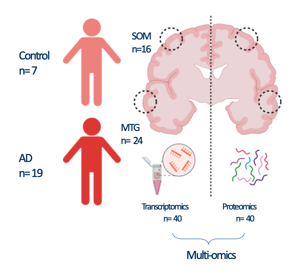
In this vignette, we proceed with a pseudotemporal multi-omics integration of 40 brain Alzheimer’s disease (AD) and Control samples coming from two brain regions

The somatosensory cortext (SOM)

The middle frontal gyrus (MTG)

The MTG is known to be affected earlier during AD progression, while SSC at later stages. Using these two regions as pseudotemporal proxi in the integrative process, we are able to gain a deeper understanding of biological mechanisms that occur during AD progression.

Pseudotemporal multi-omics integration using MOFA

multiomics_object=vertical_integration(multiassay=multiomics_object,
                                slots = c(
                                   "rna_processed",
                                   "protein_processed"
                                 ),
                                integration='MOFA',
                                ID_type = "gene_name",
                                dependent='diagnosis',
                                intersect_genes = FALSE,
                                num_factors = 15,
                                scale_views = FALSE,
                                most_variable_feature=TRUE)

The integration process is successful and all integration related object are stored in the integration slot of the multi-omics object.

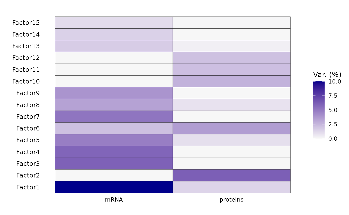
print(multiomics_object@metadata$integration$MOFA)

## Trained MOFA with the following characteristics: 
##  Number of views: 2 
##  Views names: mRNA proteins 
##  Number of features (per view): 2945 2945 
##  Number of groups: 1 
##  Groups names: group1 
##  Number of samples (per group): 40 
##  Number of factors: 15

Optional: load a pretrained model

Since package version slightly affect model outputs, we reload a pre-trained model.

multiomics_object@metadata$integration$MOFA=integrative_model

Step five - Post integration downstream analyses

Omix provides a range of built-in downstream analyses functions and visualisations. All downstream analyses will be performed on the integrated object stored in the integrated slot.

Load integrated object

integrated_object=multiomics_object@metadata$integration$MOFA
metadata=integrated_object@samples_metadata

Factor explorations

Variance explained

MOFA2::plot_variance_explained(integrated_object, max_r2=10)

Correlation of factors with covariates

integrated_object@samples_metadata$SOM=ifelse(integrated_object@samples_metadata$brain_region=='SOM',1,0)
plot=correlation_heatmap(integrated_object,
                   covariates=c("AD","Braak",'MTG','SOM',
                               'amyloid','pTau','PHF1'))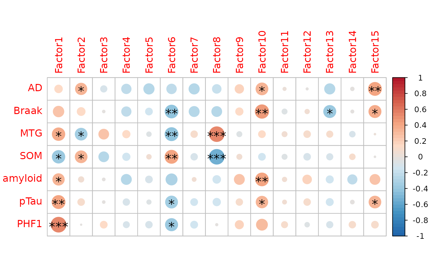

Factors 6 and 8 will be chosen for downstream analysis:

Factor 6: Is strongly correlated with neuropathological variables including PHF1 and amyloid.
Factor 8: Is strongly correlated with pseudotemporal covariates, MTG and SOM
Both share some level of variance explained by the transcriptomics and proteomics layers

Consequentially, If we project samples on these two axis of variation, we can infer on the pseudotemporal trajectory of neuropathology at the RNA and protein level.

Integrated latent space

Chosen integrated axes of variation

MOFA2::plot_factors(integrated_object,
             factors=c(8,6),
             color_by='PHF1', shape_by = 'brain_region', scale = T)+
              xlab('Factor 8 ~ Pseudotime' )+
              ylab('Factor 6 ~ Neuropathology' )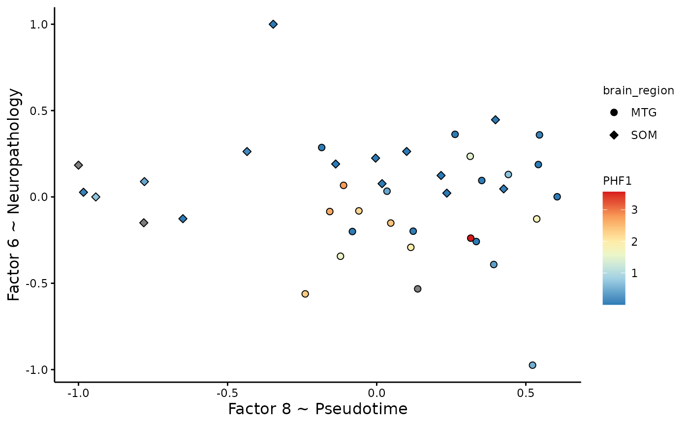

Pseudotime inference with Slingshot

The goal of slingshot (Street et al. 2017), is to use clusters of cells to uncover global structure and convert this structure into smooth lineages represented by one-dimensional variables, called “pseudotime.”

Here, we extend the use of slingshot to infer on individual level pseudotime to infer on Alzheimer’s disease trajectory.

slingshot takes a matrix of embeddings in reduced dimension as input, which here are Factors 8 and 6 from the MOFA multi-omics integration. We can optionally specify the cluster to start or end the trajectory based on biological knowledge. Here, the starting cluster should be 1 as it coincides with lowest neuropathology levels and most “recent” affected region in terms of AD trajectory.

#clusters=MOFA2::cluster_samples(integrated_object, 
#                         k=3,
#                         factors = c(8,6))

#load clusters for reproducibility
MOFA2::plot_factors(integrated_object,
             factors=c(8,6),
             color_by=clusters$cluster, scale = F)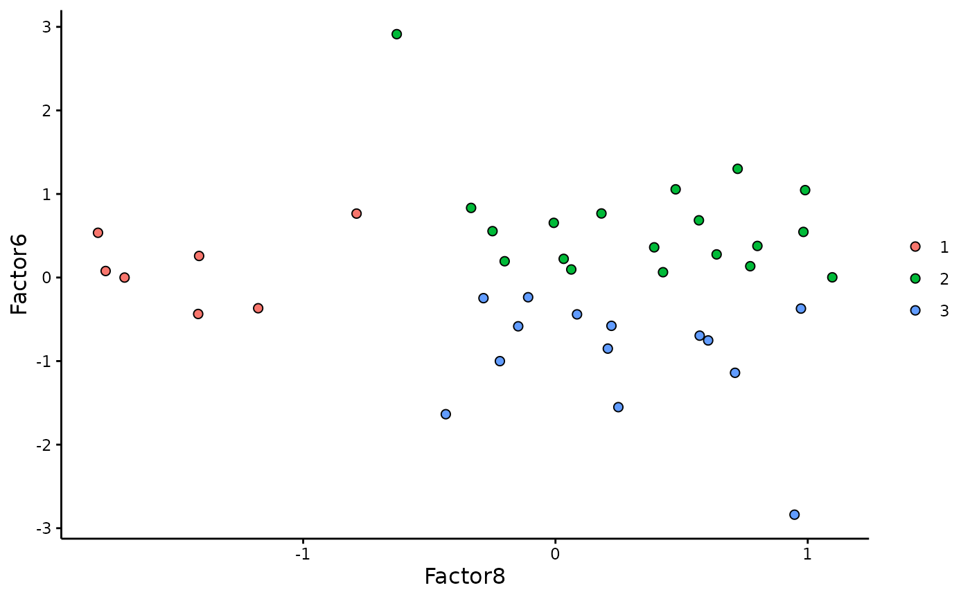

pseudotime=pseudotime_inference(integrated_object,
                                 clusters,
                                 time_factor=8,
                                 second_factor=6,
                                 start.clus = 1,
                                 end.clus=3,
                                 lineage = 'Lineage1')

pseudotime$plot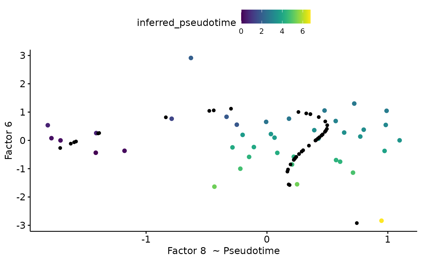

Update the integrated_object with the pseudotime

multiomics_object@metadata$integration$MOFA=pseudotime$model
integrated_object=multiomics_object@metadata$integration$MOFA
MOFA2::samples_metadata(integrated_object)$inferred_pseudotime

##  [1] 4.3991398 0.0000000 3.2695341 0.6197033 3.3734278 3.5719823 3.1405570
##  [8] 3.3321288 3.5080573 3.6197082 1.4029378 3.6919371 2.0234374 2.7175514
## [15] 2.5931510 4.3672023 1.8283014 5.2932327 4.7431202 3.4678981 4.3375355
## [22] 0.2645565 4.5626404 0.6050538 1.8689173 2.8424525 2.7175514 4.2916315
## [29] 2.6748828 4.0987023 0.1769606 4.8168531 3.0058323 3.6727096 6.7492822
## [36] 3.8811122 0.2341031 5.2714195 4.1889176 4.0515236

Extract features that are driving Factor 6 based on feature weights

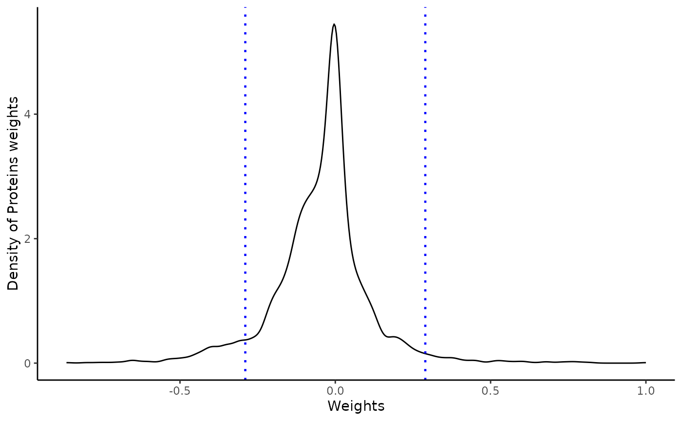
Weights vary from -1 to +1, and provide a score for how strong each feature relates to each factor, hence allowing a biological interpretation of the latent factors. Features with no association with the factor have values close to zero, while genes with strong association with the factor have large absolute values.

The sign of the weight indicates the direction of the effect:

A positive weight indicates that the feature has higher levels in the samples with positive factor values.
A negative weight indicate higher levels in samples with negative factor values.

The extract_weigthsfunction enable to extract the weights on the desired factor at a defined absolute threshold, and return an object with positive and negative weights above and below this threshold respectively. It also returns QC plots

A distribution of the feature weights for each omic layer at the designated factor
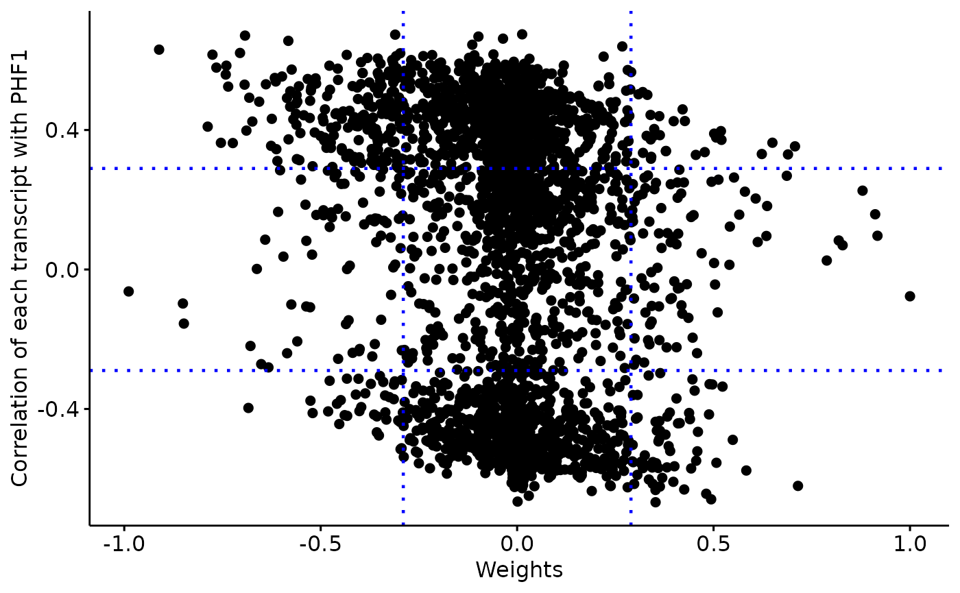
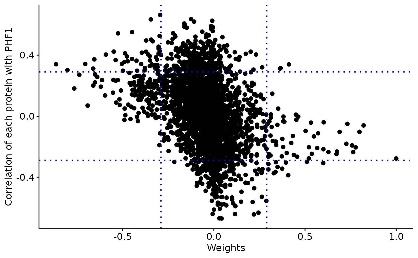
The relationship between the feature/sense_check_variable correlation and weights. High weights should coincide with stronger correlation if the sense_check_variable is an important driver of variation in the designated factor.

weights=extract_weigths(integrated_object,
                           factor=6,
                           threshold=1.5,
                           sense_check_variable='PHF1')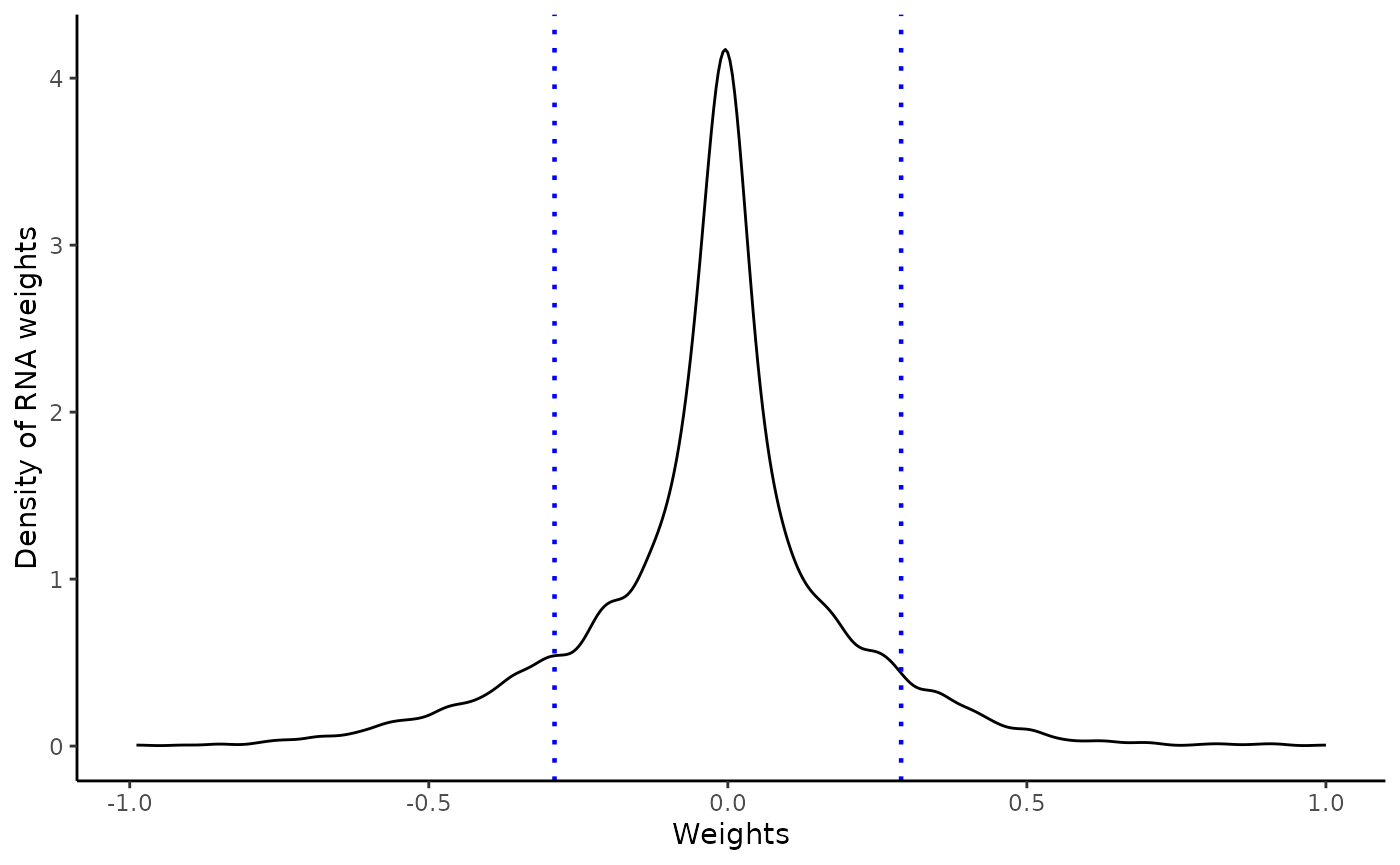

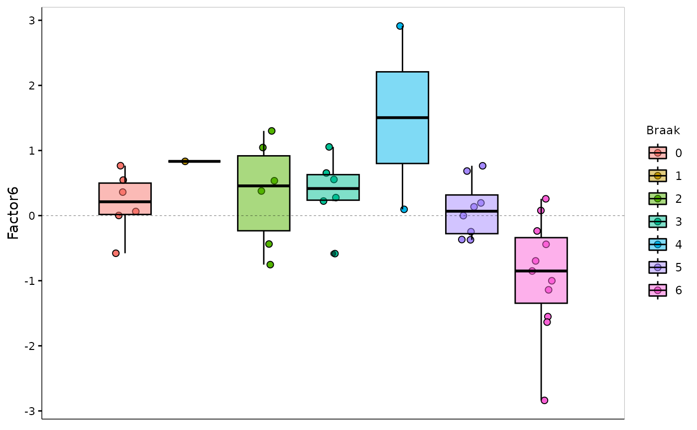
Weights distribution in Factor 6

weights$distribution_plot$rna

weights$distribution_plot$protein

Correlation to PHF1 and weights in Factor 6

weights$weights_cor_plot$rna

weights$weights_cor_plot$protein

Negative weights in factor 6: Up-regulated in later stage AD

A negative weight indicates that the feature has higher levels in the samples with negative factor values, which in this analysis coincides with later Braak stages.

integrated_object@samples_metadata$Braak=as.factor(integrated_object@samples_metadata$Braak)
MOFA2::plot_factor(integrated_object, 
            factors = 6, 
            color_by = "Braak",
            add_violin = TRUE,
            dodge = TRUE
)

Selected features based on defined threshold

rlength(weights$weights$ranked_weights_negative$rna)` RNAs have weights below -0.3 in factor 6
176 proteins have weights below -0.3 in factor 6

Some driving features may overlap between transcriptomics and proteomics

intersect(weights$weights$ranked_weights_negative$rna,weights$weights$ranked_weights_negative$protein)

##  [1] "AKAP5"   "FLNA"    "HSPG2"   "AHNAK"   "COL6A2"  "CAPG"    "TAGLN"  
##  [8] "FABP7"   "F13A1"   "C3"      "COL14A1" "ANXA2"   "C1QC"    "CRABP1" 
## [15] "DCN"     "COL1A1"  "CALB2"

7 features overlap between omic layers

Multi-omics network

Here we choose a moderate correlation threshold to draw edges between omic features (0.4)
The same analysis can be repeated with an increased correlation threshold, which will yield more modules of strongly co-expressed features.

Weights_down_n=multiomics_network(multiassay=multiomics_object,
                           list=weights$weights$ranked_weights_negative,
                           correlation_threshold =0.4,
                           filter_string_50= TRUE)

Community detection within multi-omic network

The next step of the analysis is to find densily co-expressed communities of proteins and RNAs within the multi-omics network.

This function tries to find densely connected subgraphs in a graph by calculating the leading non-negative eigenvector of the modularity matrix of the graph.

communities <- communities_network(igraph=Weights_down_n$graph,
                                    community_detection='leading_eigen')

df <- purrr::map_dfr(
    .x = communities$communities,
    .f = ~ tibble::enframe(
      x = .x,
      name = NULL,
      value = "feature"
    ),
    .id = "community"
  )

DT::datatable(
    df,
    rownames = FALSE,
    extensions = 'Buttons',
    options = list(
        dom = 'Blfrtip',
         buttons = list('colvis', list(extend = 'copy', exportOptions = list(columns=':visible')),
                                            list(extend = 'csv', exportOptions = list(columns=':visible')),
                                            list(extend = 'excel', exportOptions = list(columns=':visible')))))

5 communities are detected in the multi-omics network.
Most communities are omic dependent, since generally there is more intra omic correlation than inter omic correlation

Community detection within multi-omic network

We can look at each communities:

Community 1

community_1=community_graph(igraph=Weights_down_n$graph,
                            community_object=communities$community_object,
                            community=1)
interactive_network(igraph=community_1$graph,communities=FALSE)

Community 4

community_4=community_graph(igraph=Weights_down_n$graph,
                            community_object=communities$community_object,
                            community=4)
interactive_network(igraph=community_4$graph,communities=FALSE)

Community hubs

Features are more or less connected in the network, represented by their hub score:

print((sort(community_4$hubs, decreasing = TRUE)))

##    LY6H_protein TBC1D24_protein   RAB12_protein  CSNK1D_protein    PMM1_protein 
##      1.00000000      0.96067207      0.95018446      0.91373083      0.87930158 
##    PDK2_protein LAMTOR1_protein   ARMT1_protein ATP6AP1_protein    EIF1_protein 
##      0.85923738      0.85679461      0.83362816      0.83116292      0.82305924 
##   USP46_protein  PRUNE2_protein   C2CD5_protein    MPC2_protein    SCG2_protein 
##      0.82070521      0.81406855      0.80837977      0.79741826      0.79489801 
##    GMFG_protein   AP1S1_protein   SYNPR_protein    APEH_protein  COL1A1_protein 
##      0.78972525      0.78775116      0.77560088      0.76911869      0.73923502 
##  PRKACA_protein     POR_protein     CPE_protein   TTC7B_protein   HLA-A_protein 
##      0.72856261      0.72831672      0.71370465      0.70863268      0.69038092 
## SNRNP70_protein   SNX32_protein  CAB39L_protein     SYP_protein    GNG5_protein 
##      0.67340658      0.64531133      0.64488836      0.63591664      0.62045081 
## ALDH3A2_protein   SCN3B_protein   EXOC5_protein   SRP54_protein   MAST1_protein 
##      0.60033147      0.58197165      0.57721314      0.57670350      0.56005774 
##   ARMC8_protein   COPG1_protein   WIPI2_protein   TUBG1_protein  GABRA1_protein 
##      0.54501347      0.53781567      0.53503646      0.52329867      0.51294443 
## NECTIN1_protein   ITPR1_protein  SNRPA1_protein GUCY1A2_protein  DLGAP3_protein 
##      0.45166801      0.44363032      0.41212481      0.39655465      0.36301002 
##        C1QB_rna  ATAD3B_protein        CYBB_rna       F13A1_rna        CCR1_rna 
##      0.26034395      0.24893281      0.22441530      0.17817574      0.13574288 
##        CD14_rna        CD53_rna      CX3CR1_rna      LPCAT2_rna        LIPG_rna 
##      0.12660867      0.11629988      0.10989585      0.08313190      0.05830927 
##        PAX8_rna 
##      0.02647772

Top gene in module 4 is LY6H_protein
TREM2 or CLU, known AD risk genes expressed on microglia are present here
From prior knowledge, many of the genes in module 4 are related to microglial activation

Cell type enrichment of modules

Here we proceed with a EWCE analysis to check if modules are enriched in specific cell types.

cell_type <- cell_type_enrichment(
    multiassay =multiomics_object,
    communities = lapply(communities$communities,function(x){sub("\\_.*", "",x )}),
    ctd= ctd
  )

cell_type$plots

## $`1`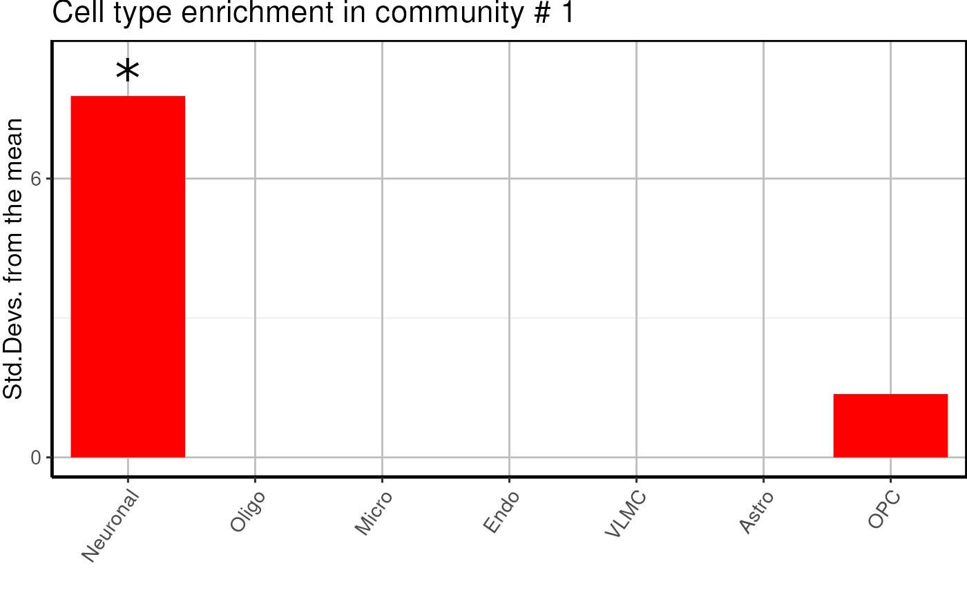

## 
## $`2`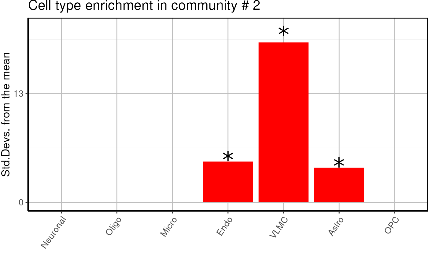

## 
## $`3`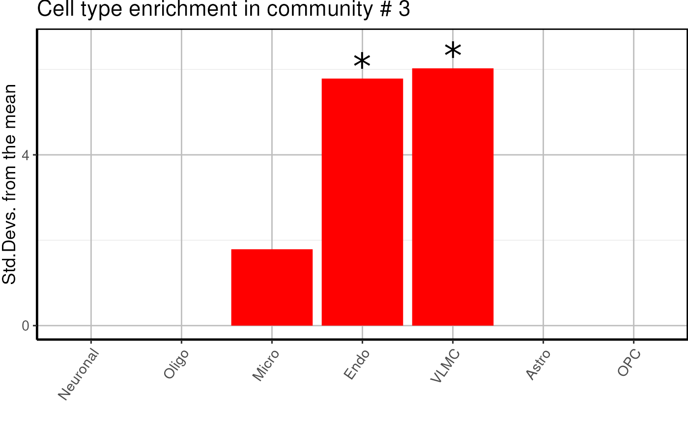

## 
## $`4`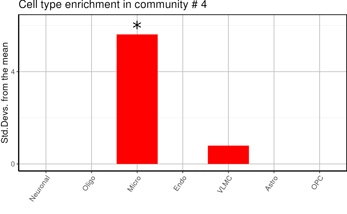

## 
## $`5`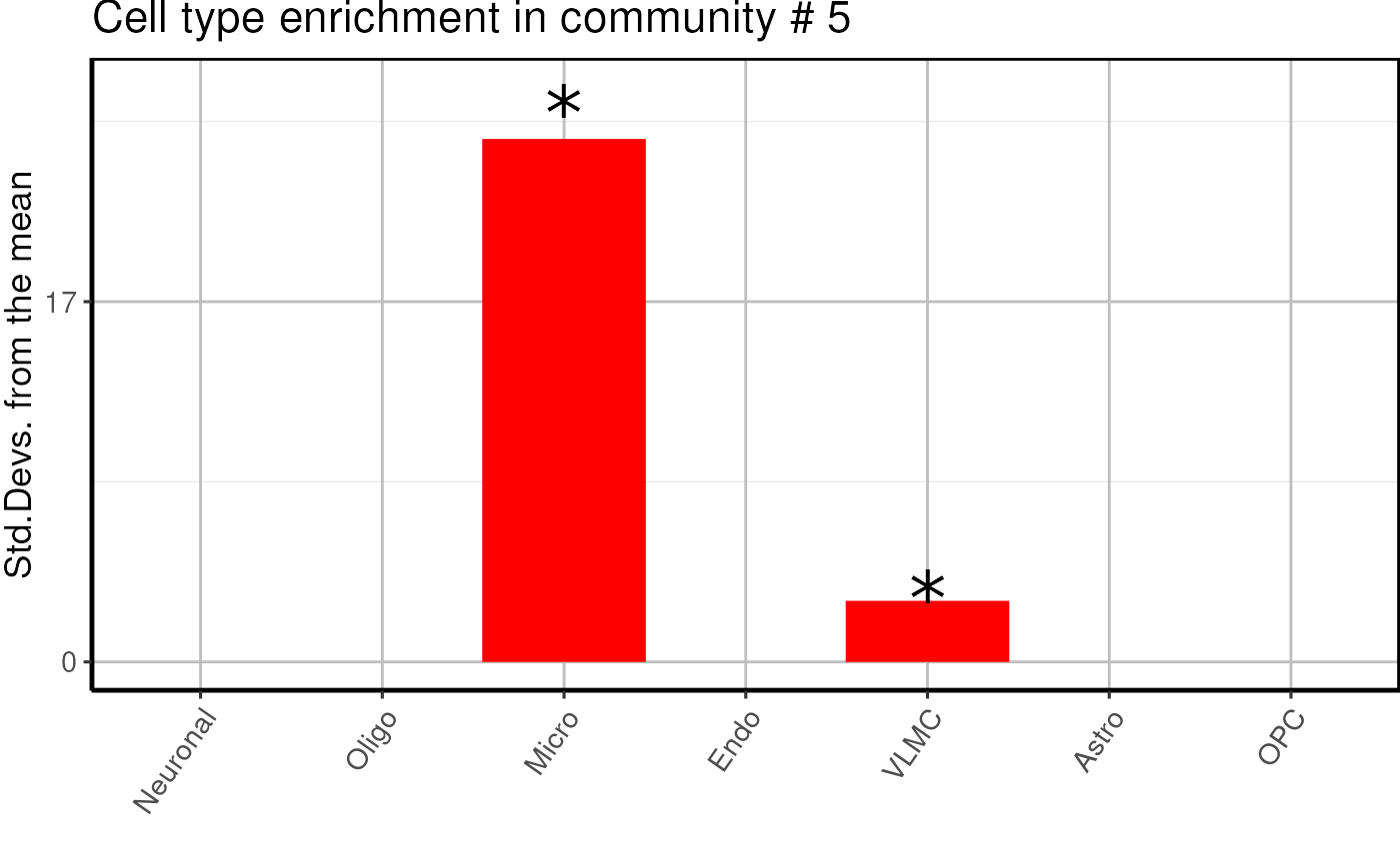

We find one neuronal, one microglial and two undefined glial enriched modules.

Pathway enrichment analysis

communities_l = lapply(communities$communities,function(x){sub("\\_.*", "",x )})

enrichment1=pathway_analysis_enrichr(communities_l$`1`,plot=5)

## Welcome to enrichR
## Checking connection ...

## Enrichr ... Connection is Live!
## FlyEnrichr ... Connection is available!
## WormEnrichr ... Connection is available!
## YeastEnrichr ... Connection is available!
## FishEnrichr ... Connection is available!

## Uploading data to Enrichr... Done.
##   Querying GO_Molecular_Function_2021... Done.
##   Querying GO_Cellular_Component_2021... Done.
##   Querying GO_Biological_Process_2021... Done.
##   Querying WikiPathways_2021_Human... Done.
##   Querying Reactome_2016... Done.
##   Querying KEGG_2021_Human... Done.
##   Querying MSigDB_Hallmark_2020... Done.
##   Querying BioCarta_2016... Done.
## Parsing results... Done.

## ℹ Output is returned as a list!

enrichment2=pathway_analysis_enrichr(communities_l$`2`,plot=5)

## Welcome to enrichR
## Checking connection ... 
## Enrichr ... Connection is Live!
## FlyEnrichr ... Connection is available!
## WormEnrichr ... Connection is available!
## YeastEnrichr ... Connection is available!
## FishEnrichr ... Connection is available!

## Uploading data to Enrichr... Done.
##   Querying GO_Molecular_Function_2021... Done.
##   Querying GO_Cellular_Component_2021... Done.
##   Querying GO_Biological_Process_2021... Done.
##   Querying WikiPathways_2021_Human... Done.
##   Querying Reactome_2016... Done.
##   Querying KEGG_2021_Human... Done.
##   Querying MSigDB_Hallmark_2020... Done.
##   Querying BioCarta_2016... Done.
## Parsing results... Done.

## ℹ Output is returned as a list!

enrichment3=pathway_analysis_enrichr(communities_l$`3`,plot=5)

## Welcome to enrichR
## Checking connection ... 
## Enrichr ... Connection is Live!
## FlyEnrichr ... Connection is available!
## WormEnrichr ... Connection is available!
## YeastEnrichr ... Connection is available!
## FishEnrichr ... Connection is available!

## Uploading data to Enrichr... Done.
##   Querying GO_Molecular_Function_2021... Done.
##   Querying GO_Cellular_Component_2021... Done.
##   Querying GO_Biological_Process_2021... Done.
##   Querying WikiPathways_2021_Human... Done.
##   Querying Reactome_2016... Done.
##   Querying KEGG_2021_Human... Done.
##   Querying MSigDB_Hallmark_2020... Done.
##   Querying BioCarta_2016... Done.
## Parsing results... Done.

## ℹ Output is returned as a list!

enrichment4=pathway_analysis_enrichr(communities_l$`4`,plot=5)

## Welcome to enrichR
## Checking connection ... 
## Enrichr ... Connection is Live!
## FlyEnrichr ... Connection is available!
## WormEnrichr ... Connection is available!
## YeastEnrichr ... Connection is available!
## FishEnrichr ... Connection is available!

## Uploading data to Enrichr... Done.
##   Querying GO_Molecular_Function_2021... Done.
##   Querying GO_Cellular_Component_2021... Done.
##   Querying GO_Biological_Process_2021... Done.
##   Querying WikiPathways_2021_Human... Done.
##   Querying Reactome_2016... Done.
##   Querying KEGG_2021_Human... Done.
##   Querying MSigDB_Hallmark_2020... Done.
##   Querying BioCarta_2016... Done.
## Parsing results... Done.

## ℹ Output is returned as a list!

enrichment5=pathway_analysis_enrichr(communities_l$`5`,plot=5)

## Welcome to enrichR
## Checking connection ... 
## Enrichr ... Connection is Live!
## FlyEnrichr ... Connection is available!
## WormEnrichr ... Connection is available!
## YeastEnrichr ... Connection is available!
## FishEnrichr ... Connection is available!

## Uploading data to Enrichr... Done.
##   Querying GO_Molecular_Function_2021... Done.
##   Querying GO_Cellular_Component_2021... Done.
##   Querying GO_Biological_Process_2021... Done.
##   Querying WikiPathways_2021_Human... Done.
##   Querying Reactome_2016... Done.
##   Querying KEGG_2021_Human... Done.
##   Querying MSigDB_Hallmark_2020... Done.
##   Querying BioCarta_2016... Done.
## Parsing results... Done.

## ℹ Output is returned as a list!

enrichment1$plot$Reactome_2016+theme(axis.text=element_text(size=12),
                                     axis.title=element_text(size=12),
                                     strip.text = element_text(size = 0, margin = margin()),
                                     legend.title = element_text(size=9))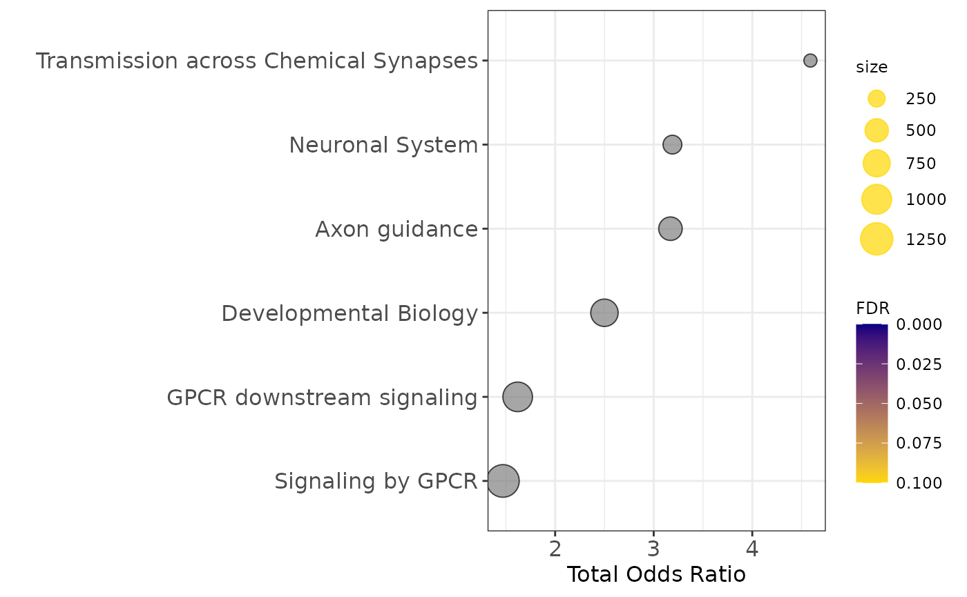

enrichment2$plot$Reactome_2016+theme(axis.text=element_text(size=12),
                                     axis.title=element_text(size=12),
                                     strip.text = element_text(size = 0, margin = margin()),
                                     legend.title = element_text(size=9))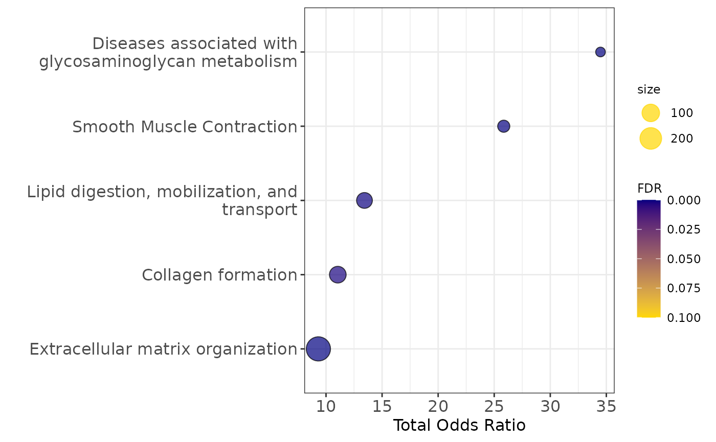

enrichment3$plot$Reactome_2016+theme(axis.text=element_text(size=12),
                                     axis.title=element_text(size=12),
                                     strip.text = element_text(size = 0, margin = margin()),
                                     legend.title = element_text(size=9))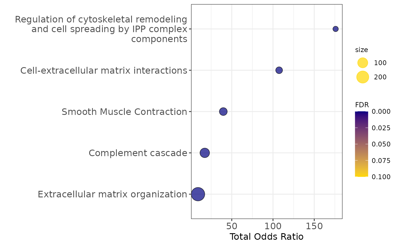

enrichment4$plot$Reactome_2016+theme(axis.text=element_text(size=12),
                                     axis.title=element_text(size=12),
                                     strip.text = element_text(size = 0, margin = margin()),
                                     legend.title = element_text(size=9))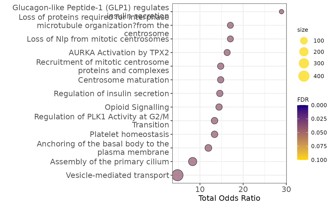

enrichment5$plot$Reactome_2016+theme(axis.text=element_text(size=12),
                                     axis.title=element_text(size=12),
                                     strip.text = element_text(size = 0, margin = margin()),
                                     legend.title = element_text(size=9))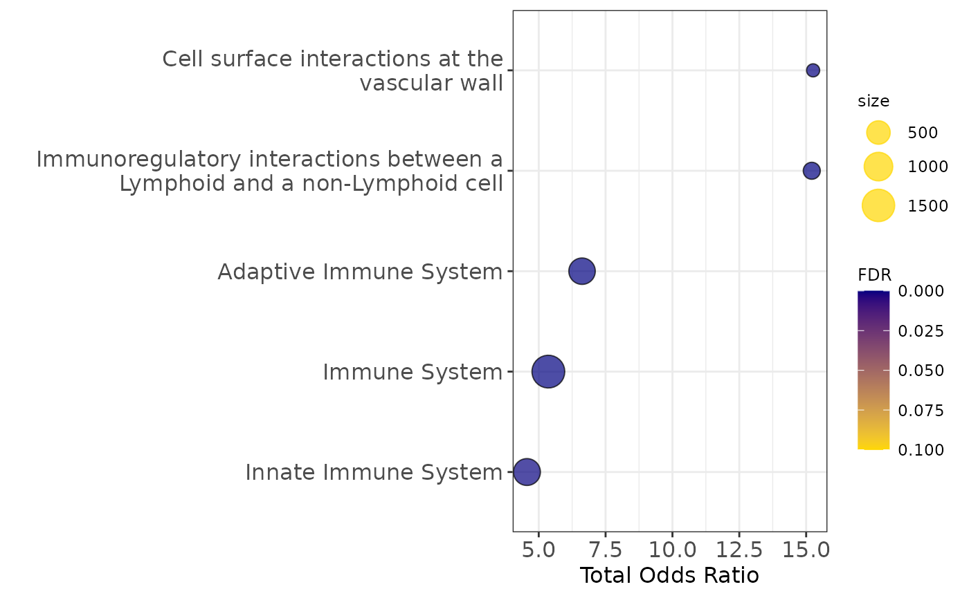

Modules correlation to neuropathology

multiomics_modules compute the module eigen value (PC1 of scaled transcriptomics/proteomics expression) and correlates it to chosen covariates

modules=multiomics_modules(multiassay=multiomics_object,
                              metadata=MOFA2::samples_metadata(integrated_object),
                              covariates=c('inferred_pseudotime','PHF1','amyloid','pTau'),
                              communities=communities$communities,
                              filter_string_50=TRUE)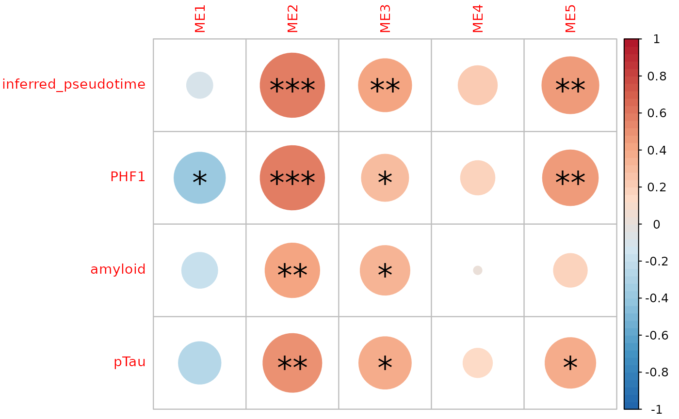

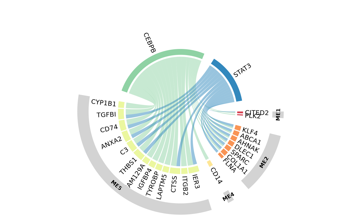
Transcription Factor - target gene enrichment

TF=Transcription_Factor_enrichment(communities=communities$communities,
                                   weights=weights,
                                   TF_gmt=TF_fp,
                                   threshold = 0.2,
                                   direction = "negative") 

GeneOverlap::drawHeatmap(TF,what = c("odds.ratio"), log.scale = T, adj.p = F, cutoff = .05,
                          ncolused = 7, grid.col = c("Blues"), note.col = "red")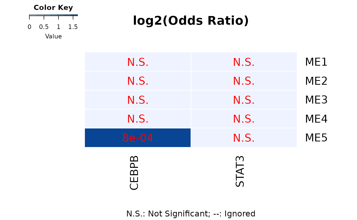

TF-target gene circos plot

circos_TF(TF)

Pseudotime ordering of multi-omics modules

Here we related each module eigen value to the pseudotime inferred from MOFA integration emmbeddings (Factors 6/8)

plot_module_trajectory(modules=modules,
                                   covariates=c('amyloid','pTau','PHF1'),
                                   plot_modules=c("ME1","ME2","ME3","ME4"))

## `geom_smooth()` using formula = 'y ~ x'
## `geom_smooth()` using formula = 'y ~ x'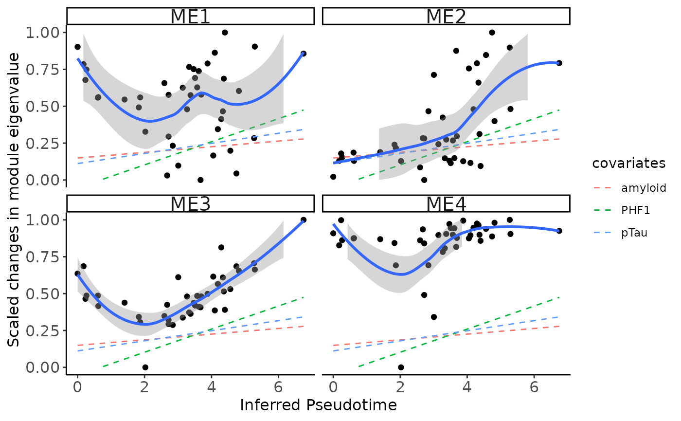

Pseudotime vs Braak

We find a stronge correlation between inferred pseudotime and PHF1, indicating that the pseudotemporal multiomics integration provides an accurate assessment of AD progression, encompassing all neuropathological measures

PHF1

modules$metadata_modules$Braak=factor(modules$metadata_modules$Braak, levels = c("0","1","2","3","4","5","6"))
modules$metadata_modules$Braak_num=as.numeric(modules$metadata_modules$Braak)
gg=ggpubr::ggscatter(modules$metadata_modules, y = "PHF1", x = "Braak_num", palette = "jco",
                     add = "reg.line", conf.int = TRUE,  label.x = 4,  add.params = list(color = "blue", fill = "lightgray"), # Customize reg. line
                     cor.coef = TRUE, # Add correlation coefficient. see ?stat_cor
                     cor.coeff.args = list(method = "pearson", label.sep = "\n"))
gb=ggpubr::ggscatter(modules$metadata_modules, y = "PHF1", x = "inferred_pseudotime", palette = "jco",
                     add = "reg.line", conf.int = TRUE,   add.params = list(color = "blue", fill = "lightgray"), # Customize reg. line
                     cor.coef = TRUE, # Add correlation coefficient. see ?stat_cor
                     cor.coeff.args = list(method = "pearson", label.x = 4, label.sep = "\n"))
plot(gg)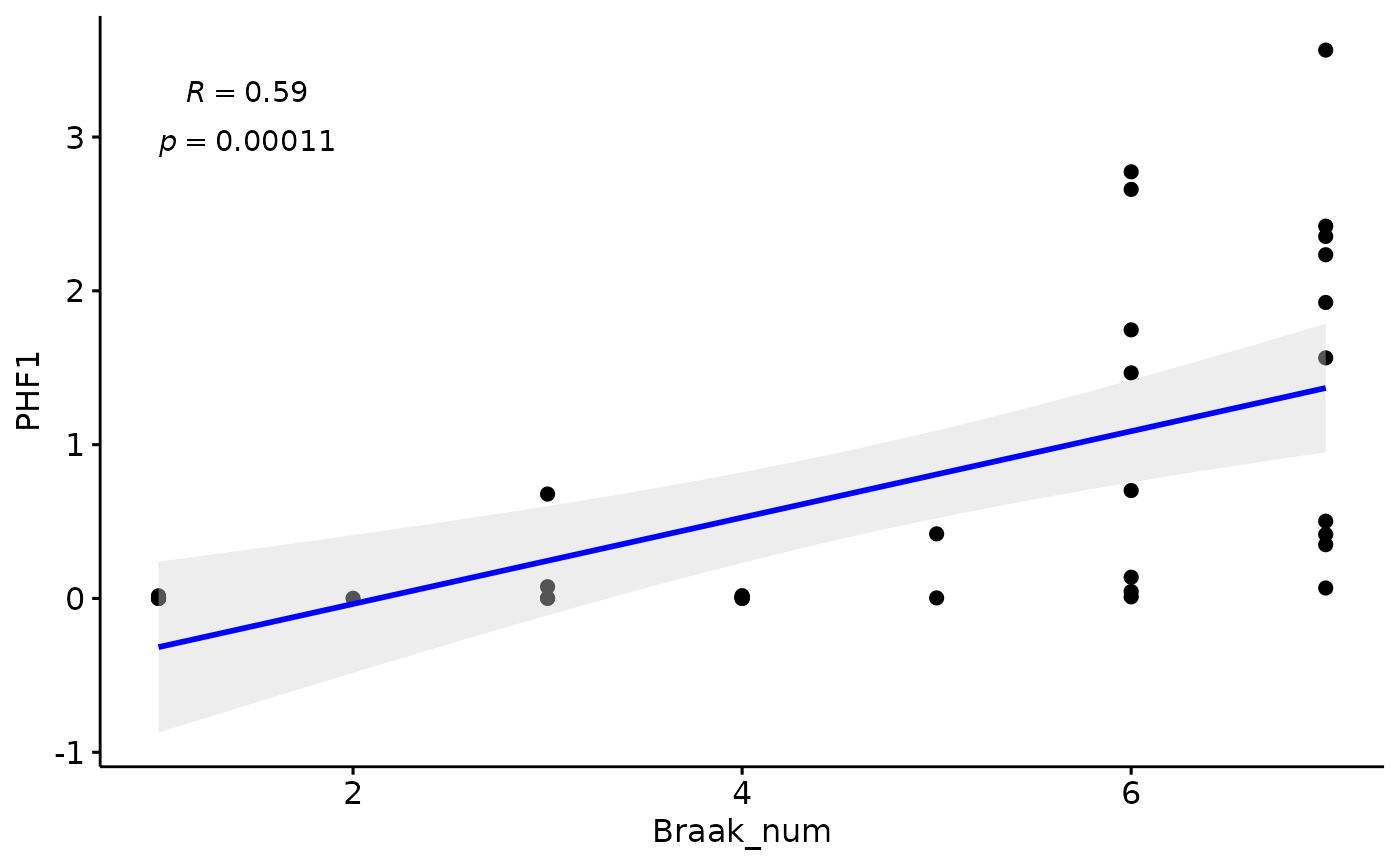

plot(gb)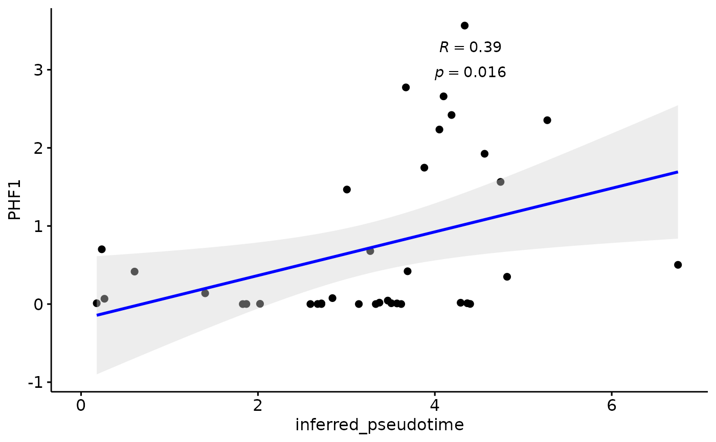

Amyloid

modules$metadata_modules$Braak=factor(modules$metadata_modules$Braak, 
                                      levels = c("0","1","2","3","4","5","6"))
modules$metadata_modules$Braak_num=as.numeric(modules$metadata_modules$Braak)
gg=ggpubr::ggscatter(modules$metadata_modules, y = "amyloid", x = "Braak_num", palette = "jco",
                     add = "reg.line", conf.int = TRUE,  label.x = 4,  add.params = list(color = "blue", fill = "lightgray"), # Customize reg. line
                     cor.coef = TRUE, # Add correlation coefficient. see ?stat_cor
                     cor.coeff.args = list(method = "pearson", label.sep = "\n"))
gb=ggpubr::ggscatter(modules$metadata_modules, y = "amyloid", x = "inferred_pseudotime", palette = "jco",
                     add = "reg.line", conf.int = TRUE,   add.params = list(color = "blue", fill = "lightgray"), # Customize reg. line
                     cor.coef = TRUE, # Add correlation coefficient. see ?stat_cor
                     cor.coeff.args = list(method = "pearson", label.x = 4, label.sep = "\n"))
plot(gg)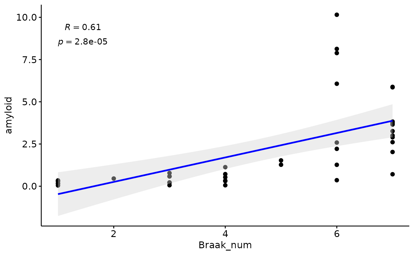

plot(gb)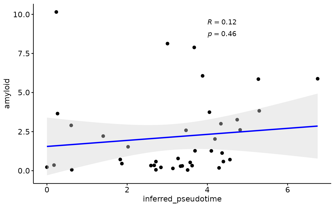

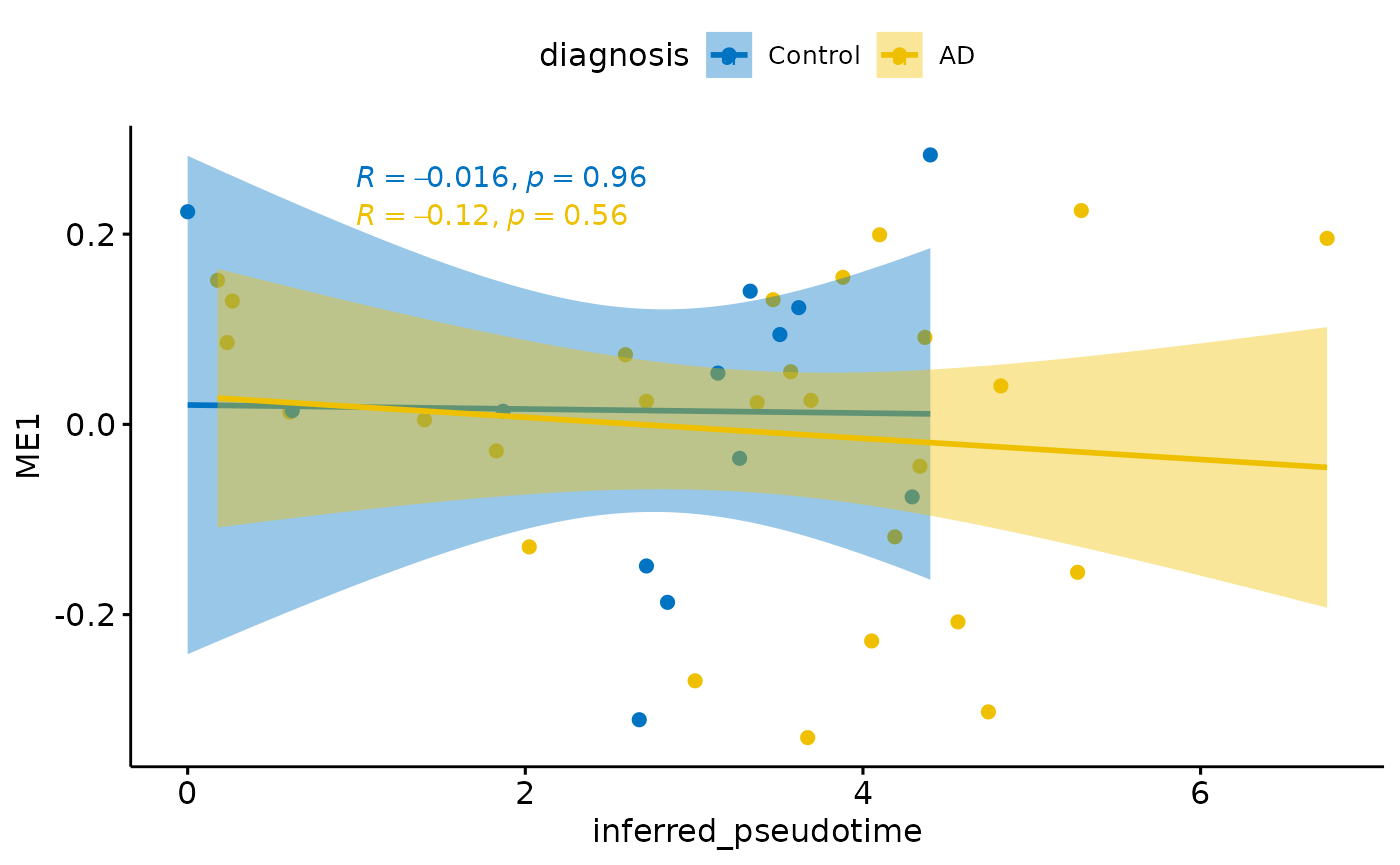
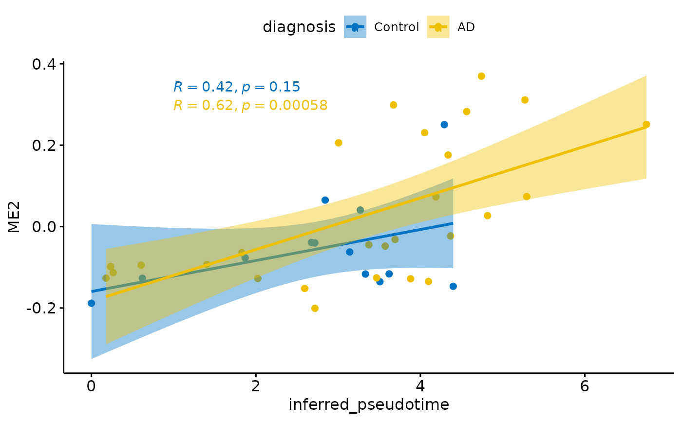
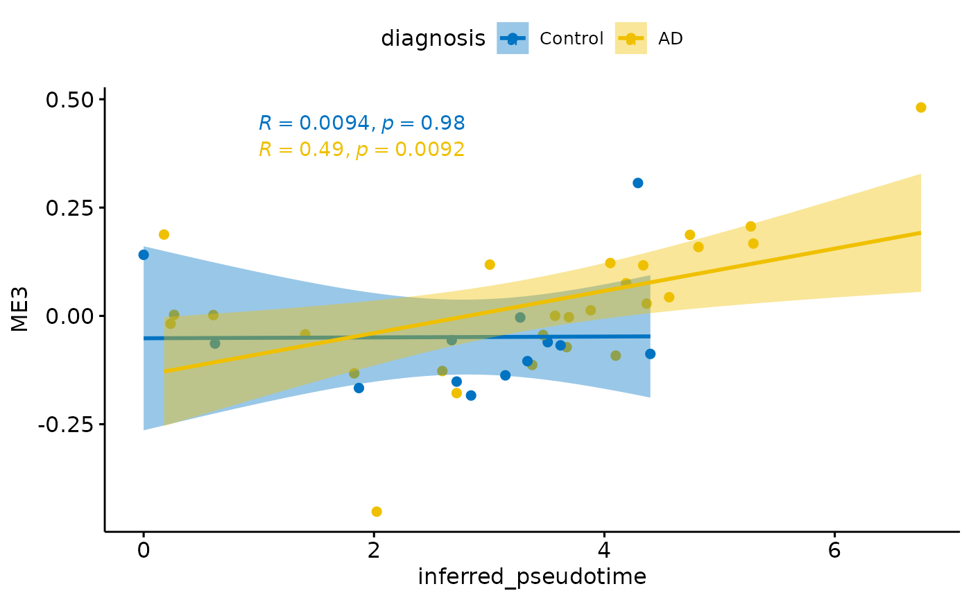
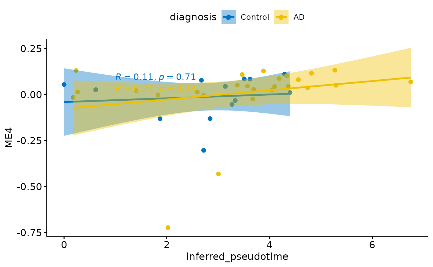
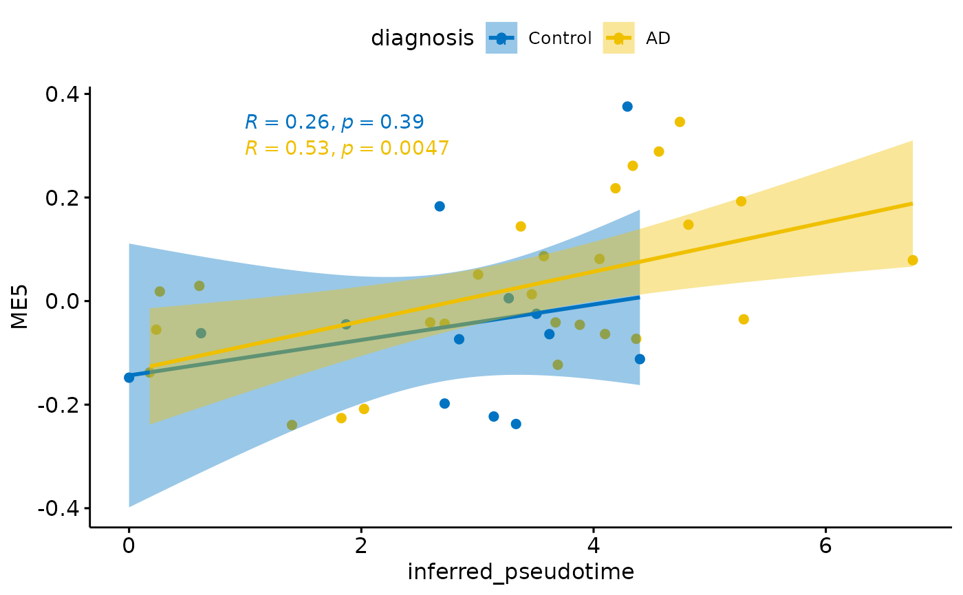
Relationship with diagnosis

for(i in colnames(modules$modules_eigen_value)){
gg=ggpubr::ggscatter(modules$metadata_modules, 
                     x = "inferred_pseudotime", 
                     y = paste(i),
          color = "diagnosis",
          palette = "jco",
          add = "reg.line", 
          conf.int = TRUE)+
  ggpubr::stat_cor(aes(color = diagnosis), label.x = 1)
plot(gg)
}

Relationship with PHF1

for(i in colnames(modules$modules_eigen_value)){
gg=ggpubr::ggscatter(modules$metadata_modules,
                     x = "PHF1", 
                     y = paste(i),
                     palette = "jco",
                     add = "reg.line", 
                     conf.int = TRUE, 
                     add.params = list(color = "blue", fill = "lightgray"), # Customize reg. line
                     cor.coef = TRUE, # Add correlation coefficient. see ?stat_cor
                     cor.coeff.args = list(method = "pearson", label.x = 2, label.sep = "\n"))


plot(gg)
}

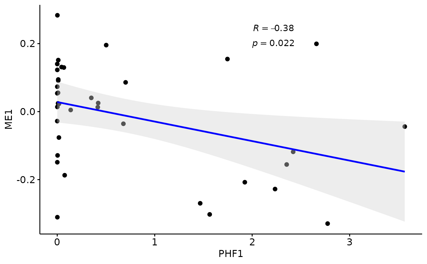
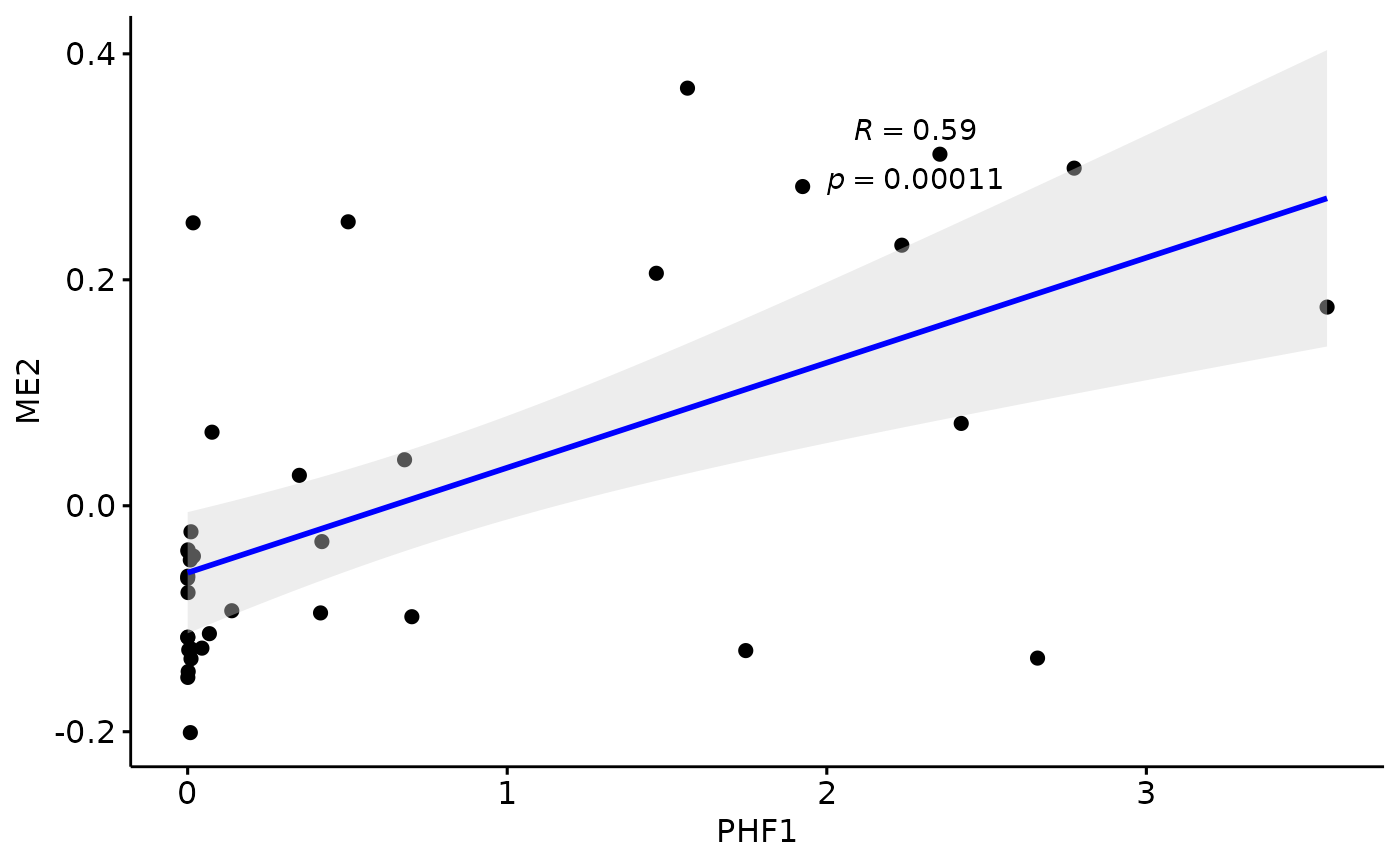
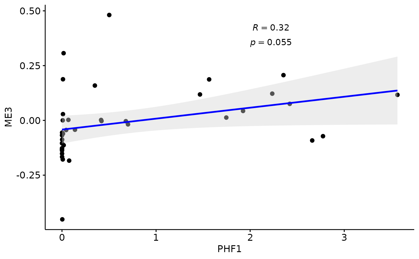
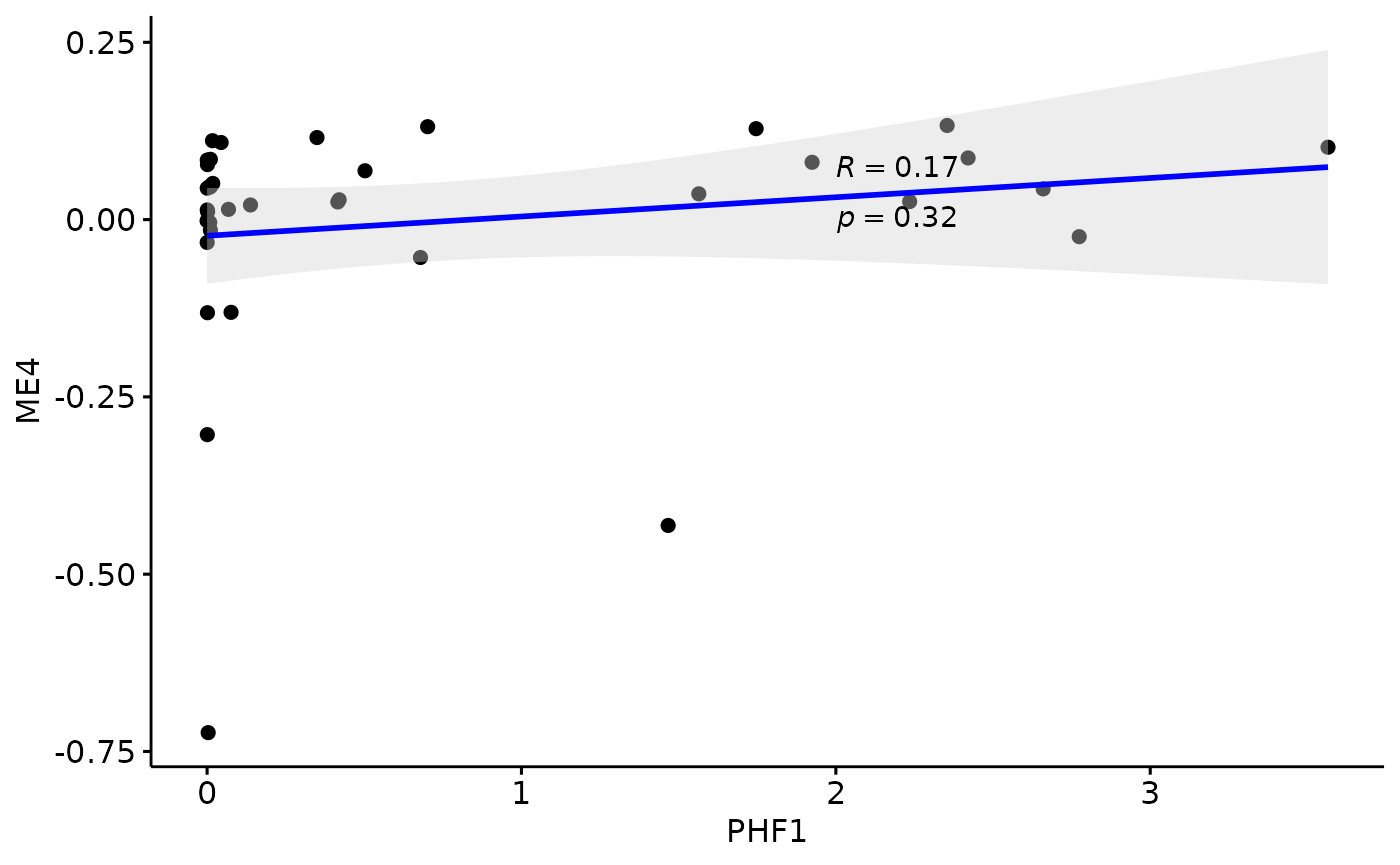
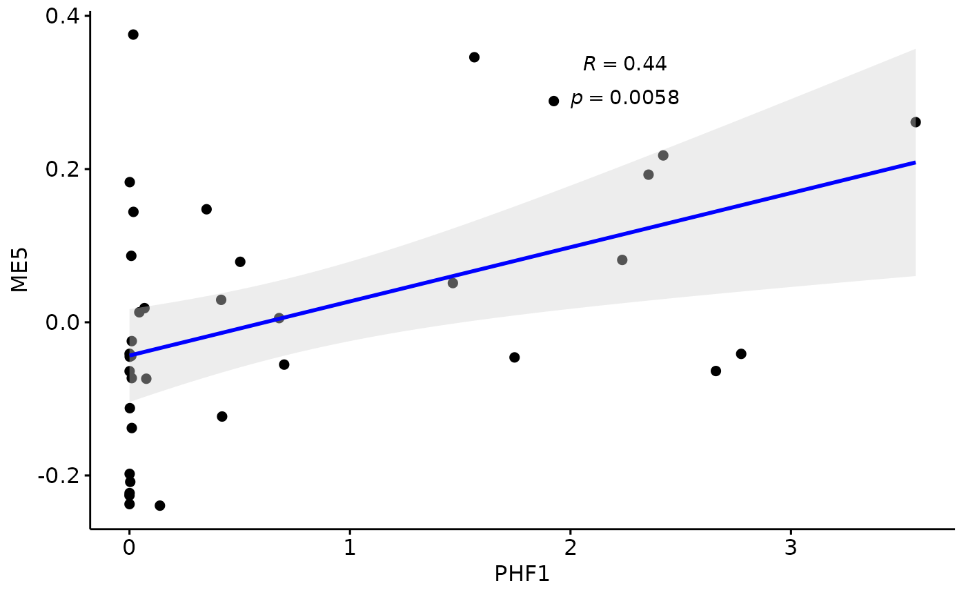
There is a stronger relationhsip between module eigen values and infered multi-omics pseudotime

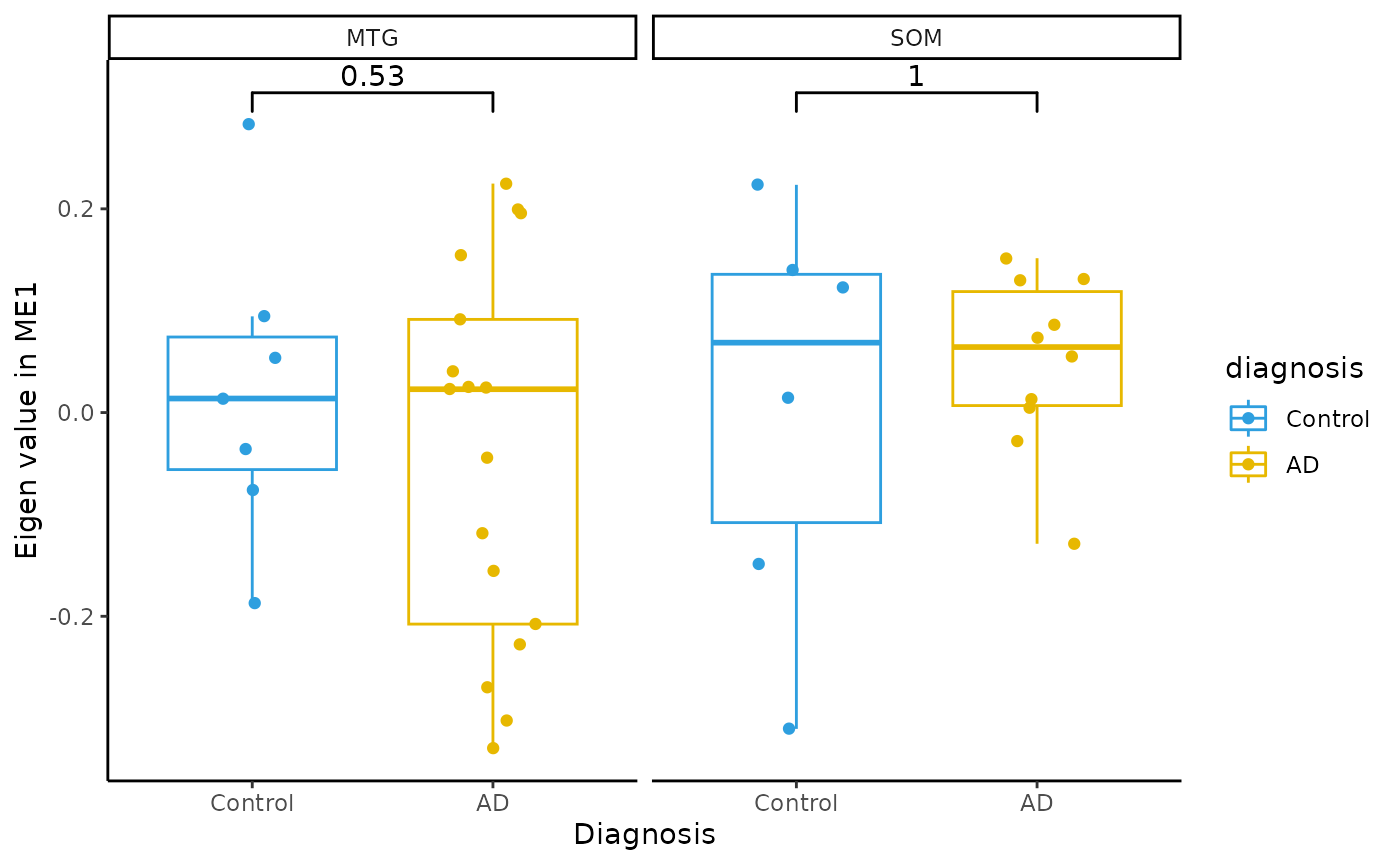
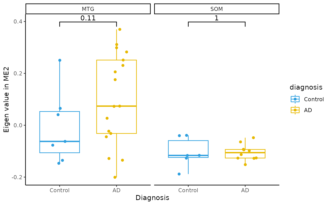
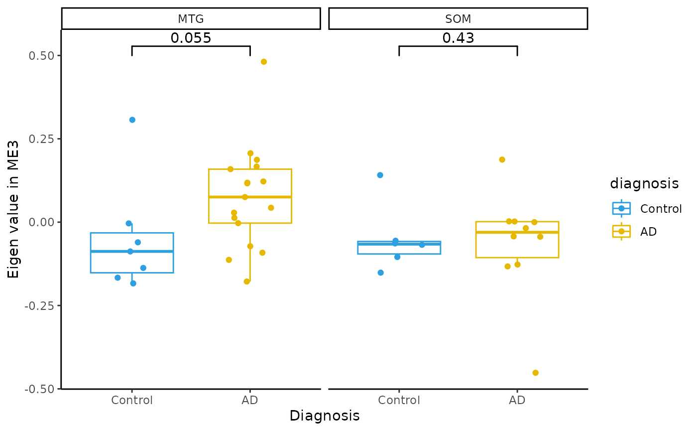
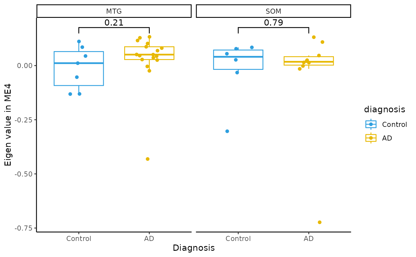
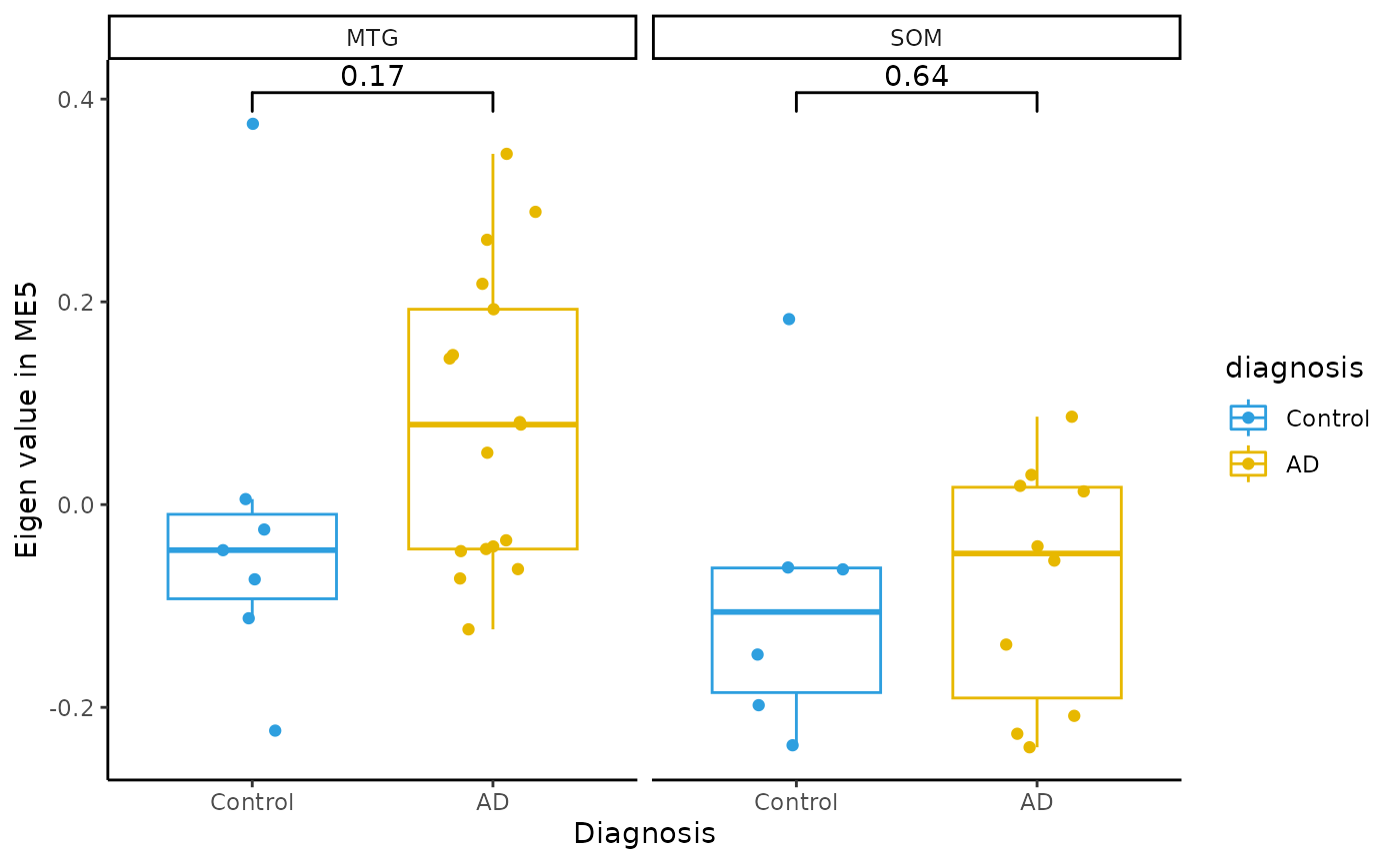
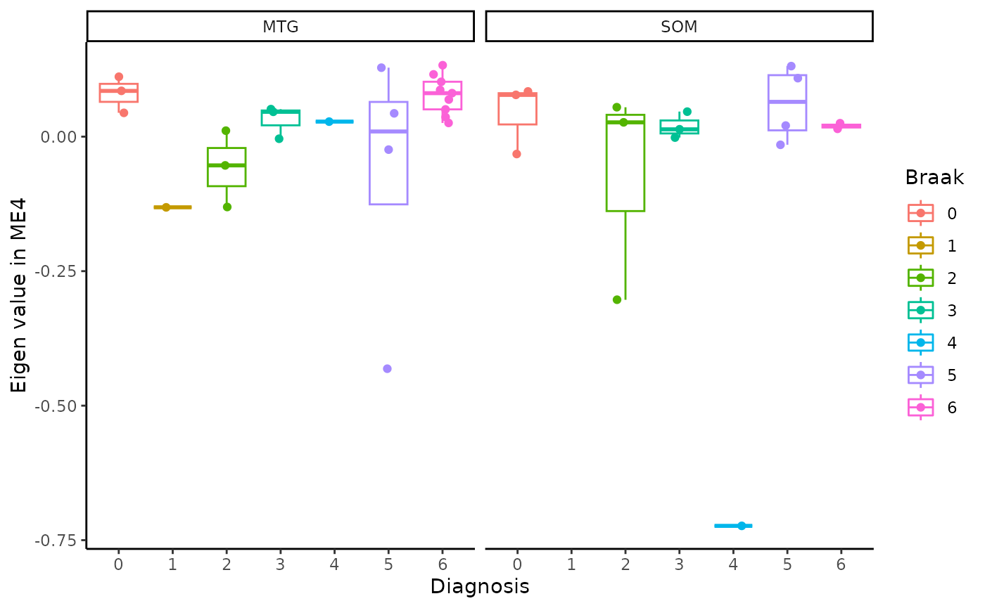
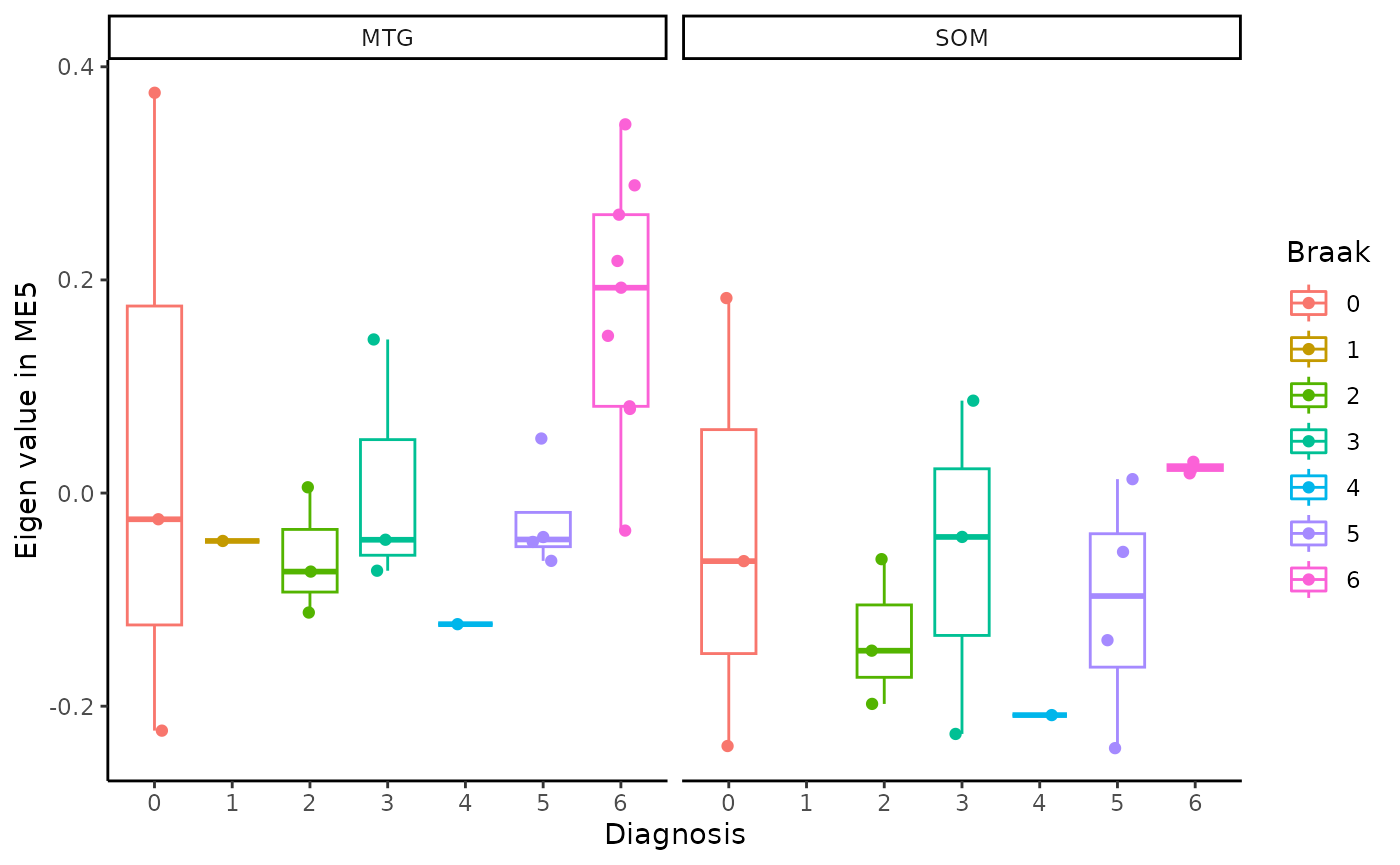
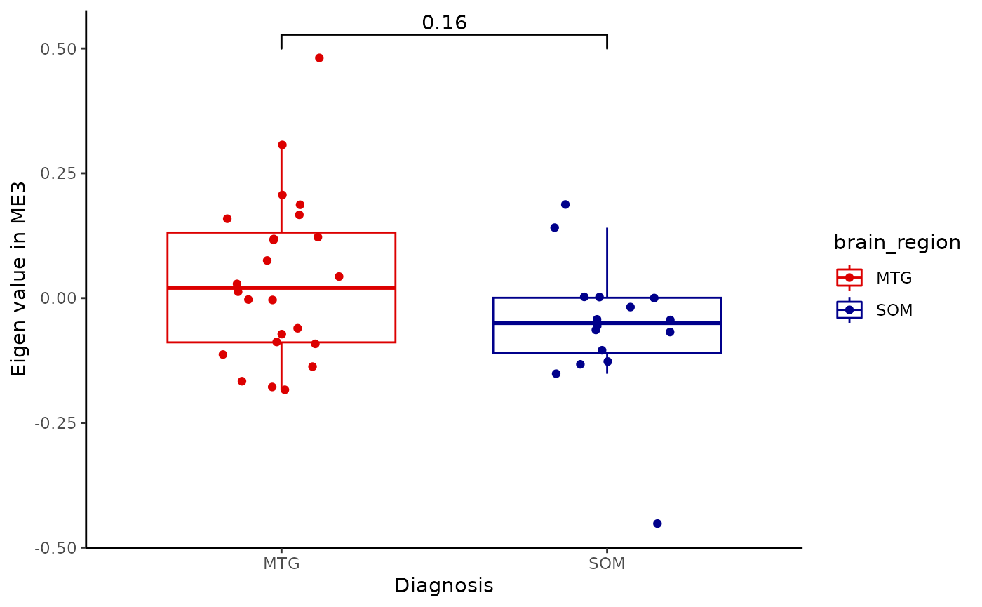
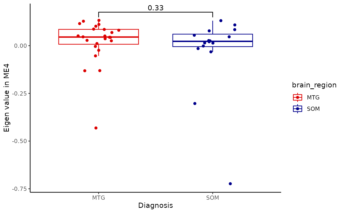
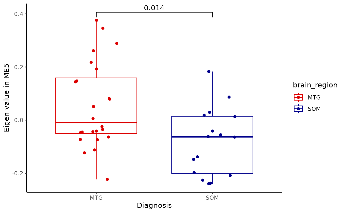
Module Eigenvalue by group boxplots

for(i in colnames(modules$modules_eigen_value)){
gg=ggpubr::ggboxplot(modules$metadata_modules,
                     x = "diagnosis", 
                     y = paste(i),
                     add='jitter', 
                     color="diagnosis")+
  xlab('Diagnosis')+
  ylab(paste('Eigen value in',i))+
  theme_classic()+
  ggsignif::geom_signif(comparisons = list(c('AD', 'Control')))+
  scale_color_manual(values = c("#2E9FDF","#E7B800"))+
  facet_wrap(~brain_region)
plot(gg)
}

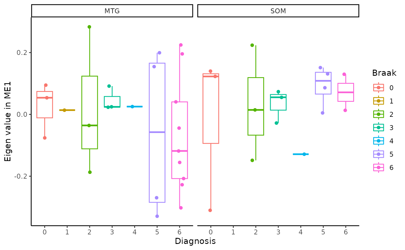
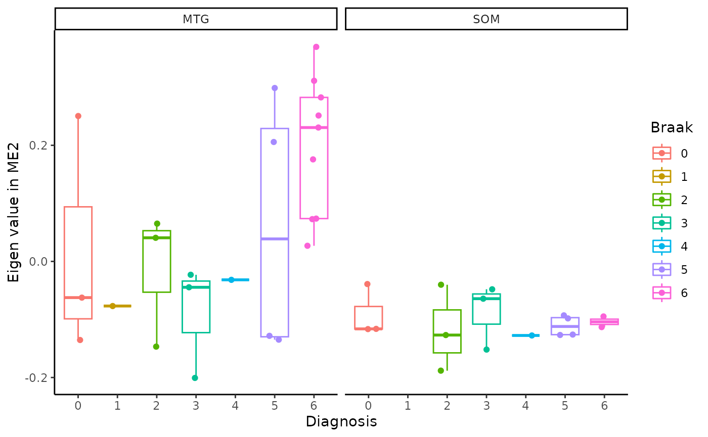
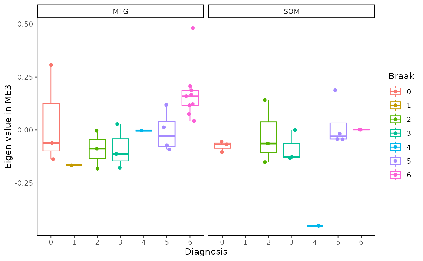
for(i in colnames(modules$modules_eigen_value)){
gg=ggpubr::ggboxplot(modules$metadata_modules, 
                     x = "Braak", 
                     y = paste(i),
                     add='jitter', 
                     color="Braak")+
  xlab('Diagnosis')+
  ylab(paste('Eigen value in',i))+
  theme_classic()+
  facet_wrap(~brain_region)
plot(gg)
}

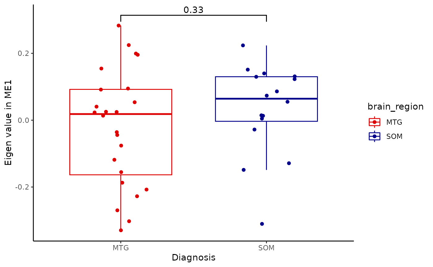
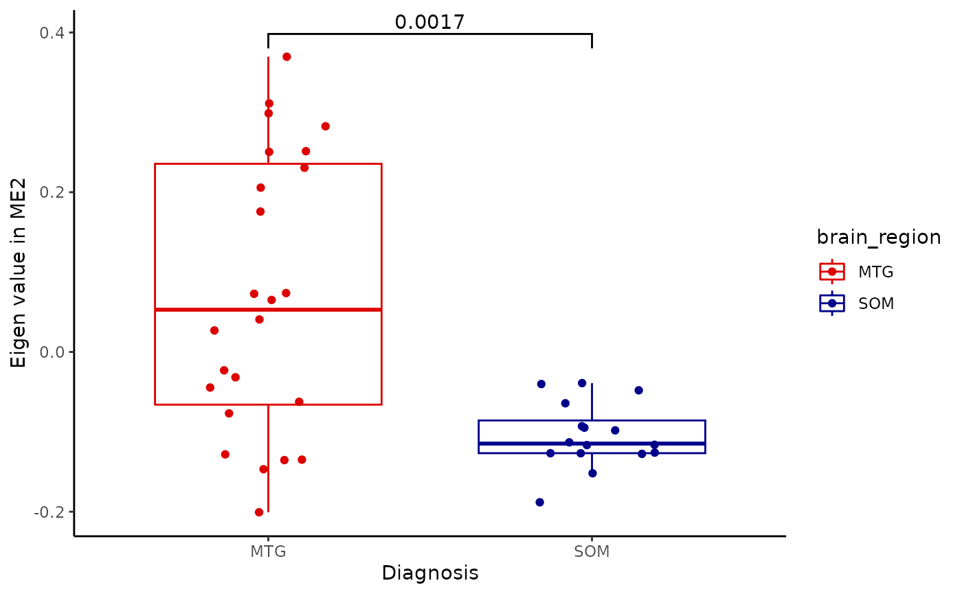
for(i in colnames(modules$modules_eigen_value)){
gg=ggpubr::ggboxplot(modules$metadata_modules, 
                     x = "brain_region", 
                     y = paste(i),
                     add='jitter',
                     color='brain_region')+
  xlab('Diagnosis')+
  ylab(paste('Eigen value in',i))+
  theme_classic()+
  ggsignif::geom_signif(comparisons = list(c('MTG', 'SOM')))+
  scale_color_manual(values = c("#DC0000FF","darkblue"))
plot(gg)
}

metadata=integrated_object@samples_metadata
ggplot(metadata, aes(x = brain_region, y = inferred_pseudotime,color=Braak)) +
  geom_point(size = 5, col = "firebrick", alpha = 0.5,aes(color=Braak)) +
  geom_line(aes(group = BBN_ID)) +
  labs(x = "Brain region", y = "Inferred_pseudotime") +
  theme_classic()+facet_wrap(~Braak)

## `geom_line()`: Each group consists of only one observation.
## ℹ Do you need to adjust the group aesthetic?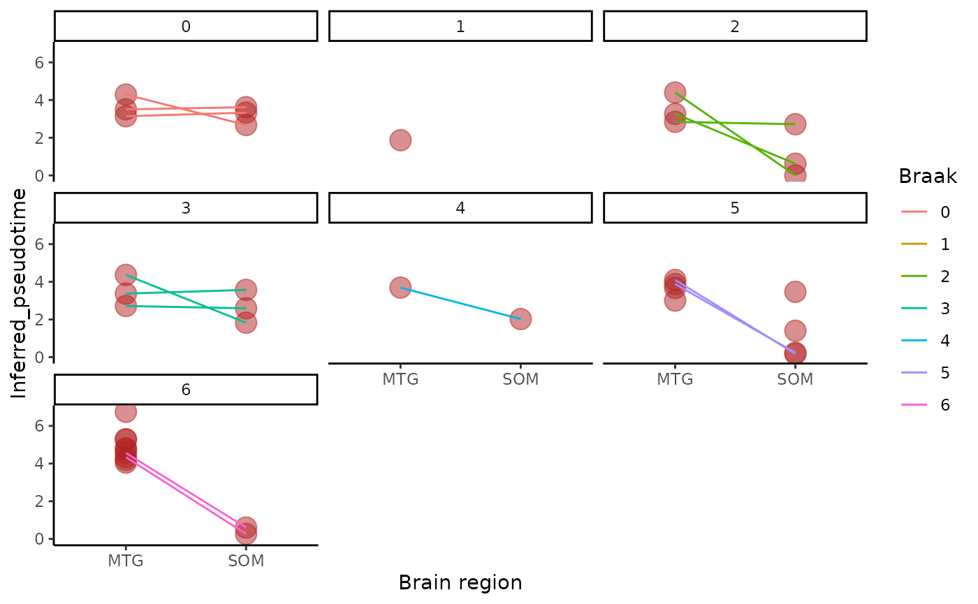

ggplot(metadata, aes(x = brain_region, y = inferred_pseudotime,color=diagnosis)) +
  geom_point(size = 5, col = "firebrick", alpha = 0.5,aes(color=Braak)) +
  geom_line(aes(group = BBN_ID)) +
  labs(x = "Brain region", y = "Inferred_pseudotime") +
  theme_classic()+facet_wrap(~diagnosis)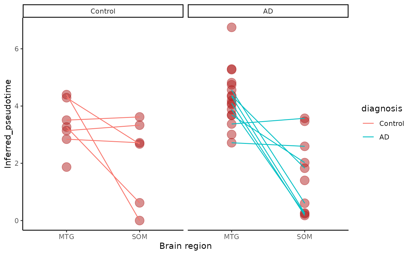

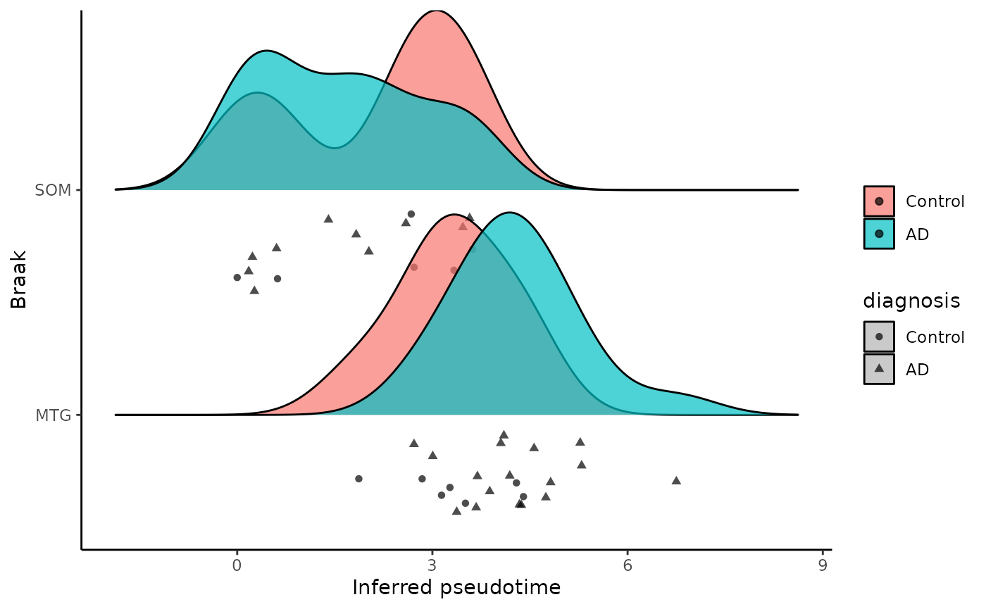
library(ggridges)
ggplot(metadata, aes(x = inferred_pseudotime, y = Braak,fill = brain_region)) +
  geom_density_ridges(aes(point_shape =diagnosis, point_fill = brain_region),
                      jittered_points = TRUE, position = "raincloud",
                      alpha = 0.7, scale = 0.9, panel_scaling=FALSE
  )+
  xlab('Inferred pseudotime')+
  ylab(paste('Braak'))+
  theme_classic()+
  labs(fill=NULL)

## Picking joint bandwidth of 0.422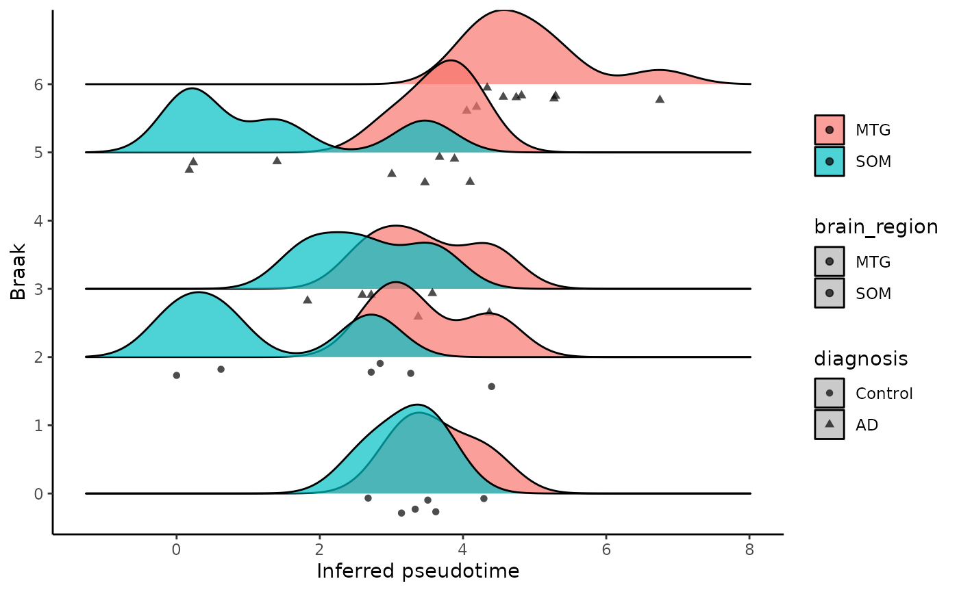

ggplot(metadata, aes(x = inferred_pseudotime, y =brain_region,fill = diagnosis)) +
  geom_density_ridges(aes(point_shape =diagnosis, point_fill = diagnosis),
                      jittered_points = TRUE, position = "raincloud",
                      alpha = 0.7, scale = 0.9, panel_scaling=FALSE
  )+
  xlab('Inferred pseudotime')+
  ylab(paste('Braak'))+
  theme_classic()+
  labs(fill=NULL)

## Picking joint bandwidth of 0.623

Omix - Pseudotemporal multi-omics integration

This vignette was created by Eléonore Schneegans and Nurun Fancy

10 April, 2024

Overview

Running Omix

Raw rna counts

Raw protein abundance

Maps

Technical metadata

Individual metadata

Optional inputs

Step one - Generate a MultiAssayExperiment object

Step two - Process transcriptomics data

Step three - Process proteomics data

Step four - Vertical integration

Pseudotemporal multi-omics integration using MOFA

Optional: load a pretrained model

Step five - Post integration downstream analyses

Load integrated object

Factor explorations

Variance explained

Correlation of factors with covariates

Integrated latent space

Chosen integrated axes of variation

Pseudotime inference with Slingshot

Update the integrated_object with the pseudotime

Extract features that are driving Factor 6 based on feature weights

Weights distribution in Factor 6

Correlation to PHF1 and weights in Factor 6

Negative weights in factor 6: Up-regulated in later stage AD

Selected features based on defined threshold

Multi-omics network

Community detection within multi-omic network

Community detection within multi-omic network

Community 1

Community 4

Community hubs

Cell type enrichment of modules

Pathway enrichment analysis

Modules correlation to neuropathology

Transcription Factor - target gene enrichment

TF-target gene circos plot

Pseudotime ordering of multi-omics modules

Pseudotime vs Braak

PHF1

Amyloid

Relationship with diagnosis

Relationship with PHF1

Module Eigenvalue by group boxplots